It’s easier to start from understanding what “gradient” means here. According to Lex Fridman at MIT, “A gradient measures how much the output of a function changes if you change the inputs a little bit.” .

Gradient descent can be thought of climbing down to the bottom of a valley. Picture if we have the valley function as f(x, y) = x^2 + xy + y^2:

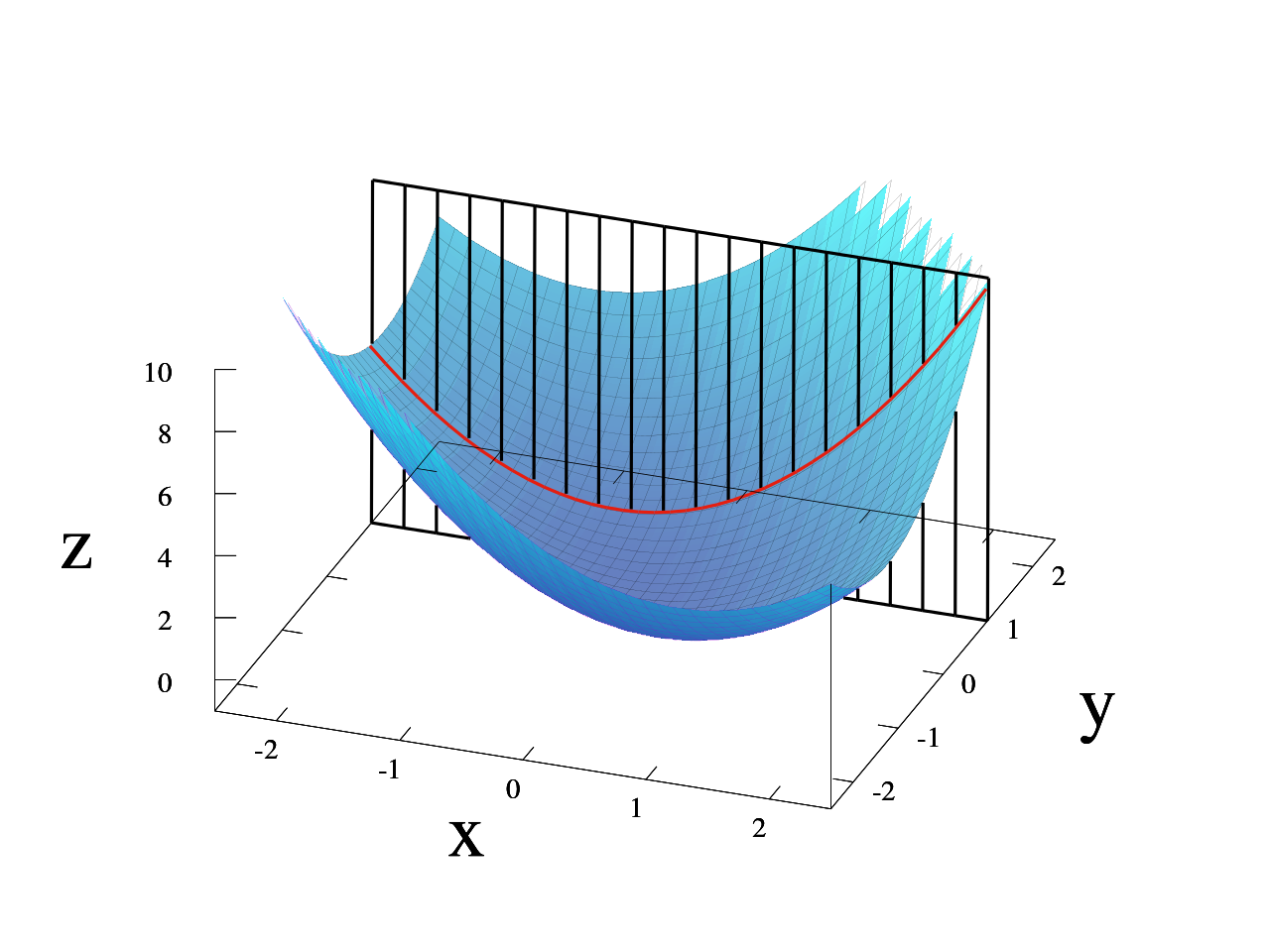
At each point in the valley, you want to find the steepest path to the bottom. The equation is

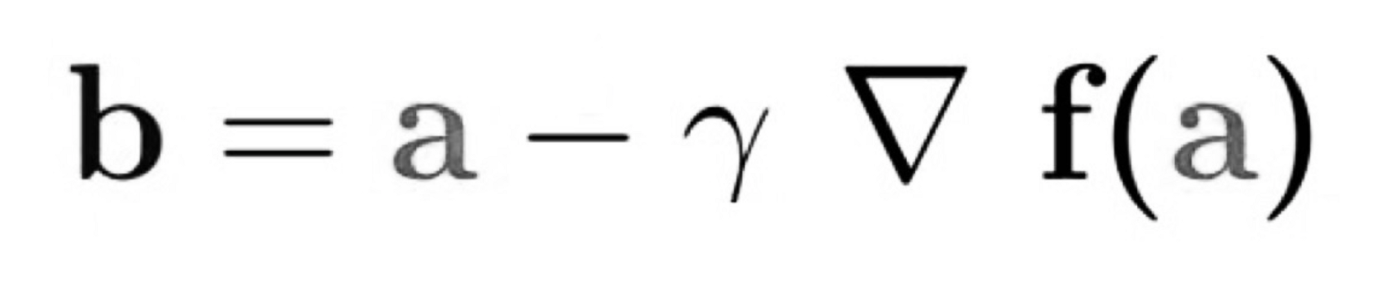
b“ describes the next position of our climber, while „a“ represents his current position. The minus sign refers to the minimization part of gradient descent. The „gamma“ in the middle is a waiting factor and the gradient term ( Δf(a) ) is simply the direction of the steepest descent.

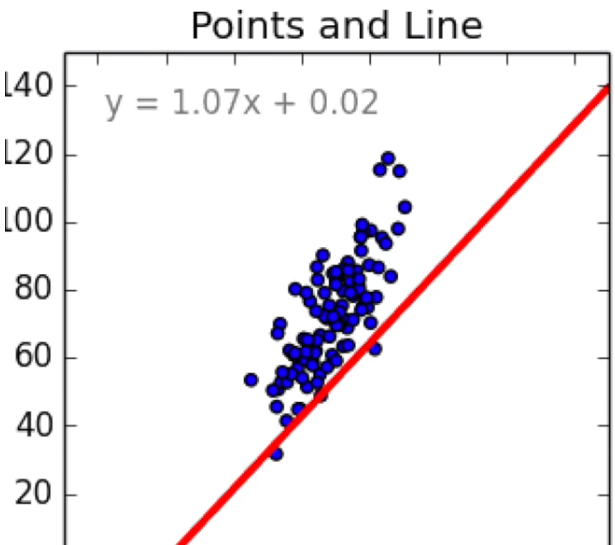
In applying Gradient Descent, let’s use an even more simple example, (from Siraj Raval), the purpose is to find the most approximate line to fit these bunch of points:

#The optimal values of m and b can be actually calculated with way less effort than doing a linear regression.
#this is just to demonstrate gradient descent

from numpy import *

# y = mx + b
# m is slope, b is y-intercept
def compute_error_for_line_given_points(b, m, points):
totalError = 0
for i in range(0, len(points)):
x = points[i, 0]
y = points[i, 1]
totalError += (y – (m * x + b)) ** 2
return totalError / float(len(points))

def step_gradient(b_current, m_current, points, learningRate):
b_gradient = 0
m_gradient = 0
N = float(len(points))
for i in range(0, len(points)):
x = points[i, 0]
y = points[i, 1]
b_gradient += -(2/N) * (y – ((m_current * x) + b_current))
m_gradient += -(2/N) * x * (y – ((m_current * x) + b_current))
new_b = b_current – (learningRate * b_gradient)
new_m = m_current – (learningRate * m_gradient)
return [new_b, new_m]

def gradient_descent_runner(points, starting_b, starting_m, learning_rate, num_iterations):
b = starting_b
m = starting_m
for i in range(num_iterations):
b, m = step_gradient(b, m, array(points), learning_rate)
return [b, m]

def run():
points = genfromtxt(“data.csv”, delimiter=”,”)
learning_rate = 0.0001
initial_b = 0 # initial y-intercept guess
initial_m = 0 # initial slope guess
num_iterations = 1000
print “Starting gradient descent at b = {0}, m = {1}, error = {2}”.format(initial_b, initial_m, compute_error_for_line_given_points(initial_b, initial_m, points))
print “Running…”
[b, m] = gradient_descent_runner(points, initial_b, initial_m, learning_rate, num_iterations)
print “After {0} iterations b = {1}, m = {2}, error = {3}”.format(num_iterations, b, m, compute_error_for_line_given_points(b, m, points))

if __name__ == ‘__main__’:
run()

So we start from the initial values m = 0, b = 0, plugging in y = m + b*x, b_gradient and m_gradient are also initialized as 0, then “partial derivative” is applied, which is slope relative to the two variable m and b respectively.

    b_gradient += -(2/N) * (y - ((m_current * x) + b_current))
    m_gradient += -(2/N) * x * (y - ((m_current * x) + b_current))

Then there is another concept – learning rate, how tiny steps you would take to iterate, neither too high nor too low rate is ideal, there is an optimal rate.