Hidden markov model is suitable for data that contains States, Observation Distribution and Transition Distribution. The weather data is ideal to use here, specifically,

1. Cold days are encoded by a 0 and hot days are encoded by a 1.
2. The first day in our sequence has an 80% chance of being cold.
3. A cold day has a 30% chance of being followed by a hot day.
4. A hot day has a 20% chance of being followed by a cold day.
5. On each day the temperature is normally distributed with mean and standard deviation 0 and 5 on a cold day and mean and standard deviation 15 and 10 on a hot day.

However you can see this is less like the typical ML model where a large training data is fed, and then evaluation data to test accuracy, in this model, it’s more like a rule based math calculation.

tfd = tfp.distributions

# A simple weather model.

# Represent a cold day with 0 and a hot day with 1.
# Suppose the first day of a sequence has a 0.8 chance of being cold.

initial_distribution = tfd.Categorical(probs=[0.8, 0.2])

# Suppose a cold day has a 30% chance of being followed by a hot day
# and a hot day has a 20% chance of being followed by a cold day.

transition_distribution = tfd.Categorical(probs=[[0.7, 0.3],
                                                 [0.2, 0.8]])

# Suppose additionally that on each day the temperature is
# normally distributed with mean and standard deviation 0 and 5 on
# a cold day and mean and standard deviation 15 and 10 on a hot day.

observation_distribution = tfd.Normal(loc=[0., 15.], scale=[5., 10.])

# This gives the hidden Markov model:

model = tfd.HiddenMarkovModel(
    initial_distribution=initial_distribution,
    transition_distribution=transition_distribution,
    observation_distribution=observation_distribution,
    num_steps=7)

# Suppose we observe gradually rising temperatures over a week:
temps = [-2., 0., 2., 4., 6., 8., 10.]

# We can now compute the most probable sequence of hidden states:

model.posterior_mode(temps)

# The result is [0 0 0 0 0 1 1] telling us that the transition
# from "cold" to "hot" most likely happened between the
# 5th and 6th days.

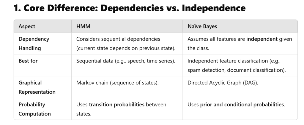
Both Hidden Markov Models (HMMs) and Naïve Bayes (NB) classifiers are probabilistic models used in classification, but they differ significantly in how they handle dependencies, sequential data, and probabilistic assumptions. Below is an intuitive and technical comparison.

traditional classifiers like HMM, Naive Bayes, SVM, K-Means, and Random Forest have all been surpassed by neural networks. Let me start by breaking down each of these classifiers and their use cases.

First, I need to recall what each of these models does. HMM is for sequential data, Naive Bayes is probabilistic and good for text, SVM works well with high-dimensional data, K-Means is clustering, and Random Forest is an ensemble method. Neural networks, especially deep learning, have become very popular, but are they replacing all these?

Ensemble learning is a machine learning paradigm where multiple models (learners) are combined to solve a problem, often outperforming any single model. Think of it like consulting a team of experts instead of relying on one person—their collective judgment is usually more robust and accurate. Example of Ensemble learnings:

1. Random Forest
   • Uses bagging with decision trees. Each tree votes, and the majority wins.
   • Robust to noise, handles high-dimensional data.
2. Gradient Boosting (XGBoost, LightGBM)
   • Sequentially corrects errors using gradient descent.
   • Dominates Kaggle competitions for structured/tabular data.
3. Stacked Generalization
   • Base models (e.g., SVM, k-NN) make predictions → meta-model (e.g., logistic regression) learns to combine them.