Second order harmonic oscillator, characteristic equation, ode45, following the first review 01, typical example of spring movement governed by Newton’s law, physicist wants to solve the equation, they always start with guessing, even famous theories such as general relativity and quantum mechanics, essentially are guess work.

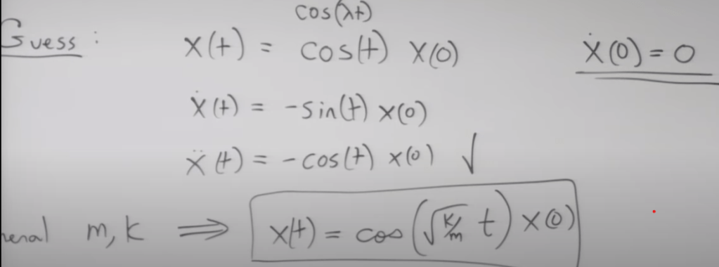
So to solve this harmonic spring oscillation problem, method 1, guess it’s a cosine wave function:

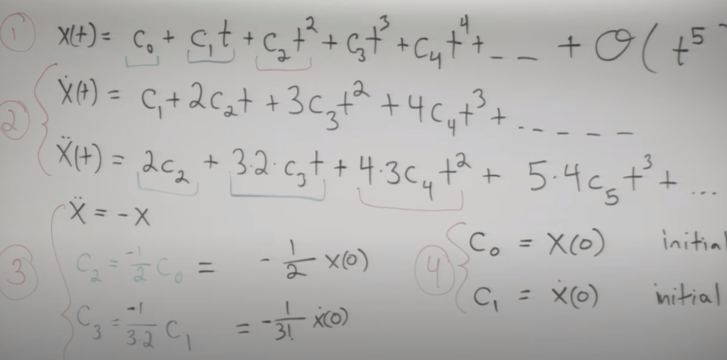
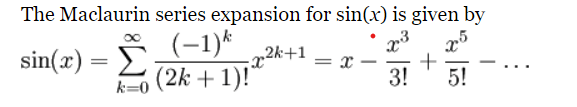
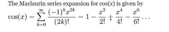
Method2, use Taylor Series

Follow the steps as

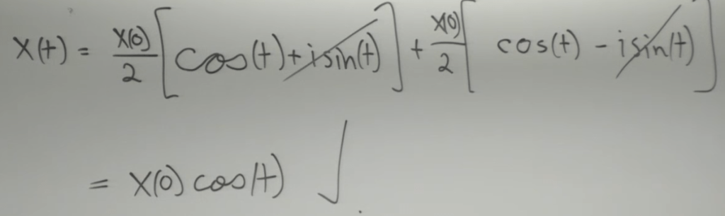
then deduce a more accurate equation: X(t) = cos(t)X(0) + sin(t)X(0)’

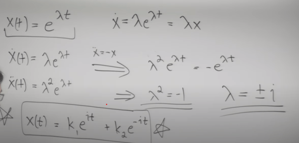
Method 3, take a guess again. What function satisfy X” = X, it looks like that e raised to t time lambda, so plug it in to figure out lambda

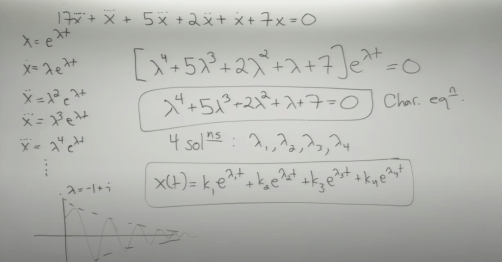
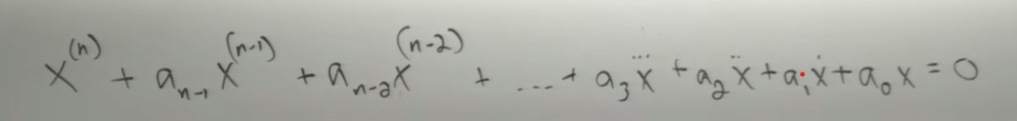
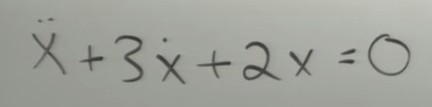
This method is powerful to solve linear higher ODE for example

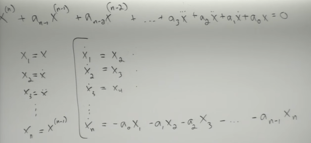
To plug in computer we need to reduce this one line higher order equation to multiple first order DE as

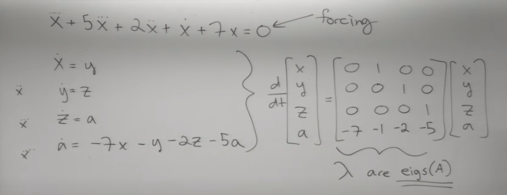
Geometrically the eigenvalues of A is the four solutions of lambda. (try to connect these two…), a.k.a

He starts from the generic form of higher order linear ODE

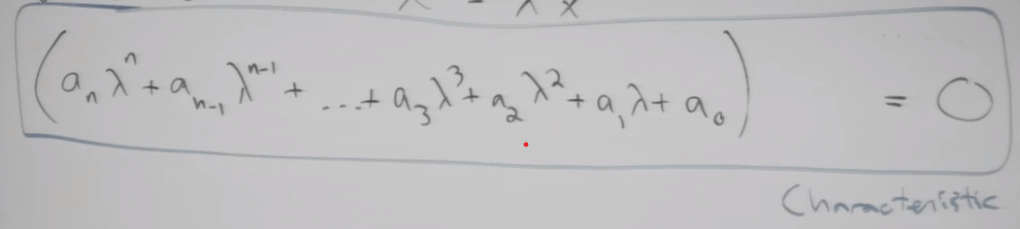
Then deduce the above equation which is called characteristic polynomial. Knowing the word stem of “characteristic” in German is “eigen”, we know why lambda are mathematically called “eigenvalue, eigenvectors” now.

System of all first order ODEs,

Then we need to rewrite in matrix form, before that, I’d like to go over dot product of matrices

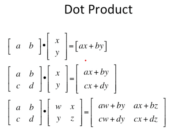
so now it’s easy to understand how we can rewrite the reduced series of first order ODEs into

in a more general form, it can be written as y’ = A * y

Further, let’s use a simpler example to have a deep understanding

Then we conclude the eigenvalues of A is the solution for this simple ODE.

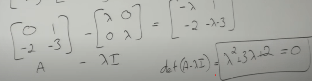
If in angular motion, the equation is as follows, question on why A left bottom corer is 1?

Why?

First, calculate the eigenvalues of A by

To compute the determinate of A-lambda*I

Next, we want to generalize it

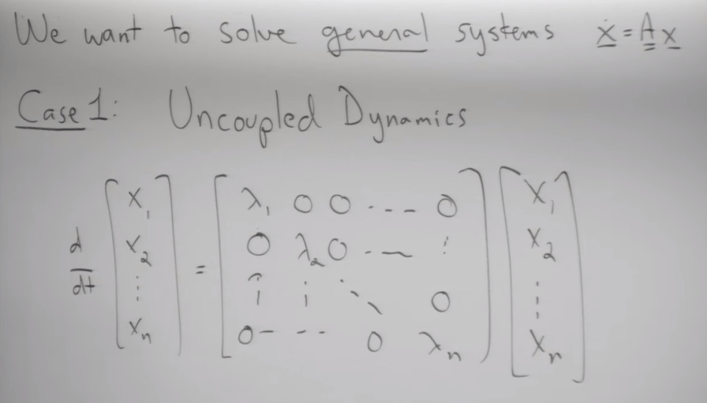
the solution can also be written in matrix form as

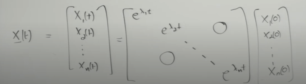
And further shorthand, written as

Mathematicians realized it’s important to find coordinate transformation to turn diagonal, so here is the ingenious step

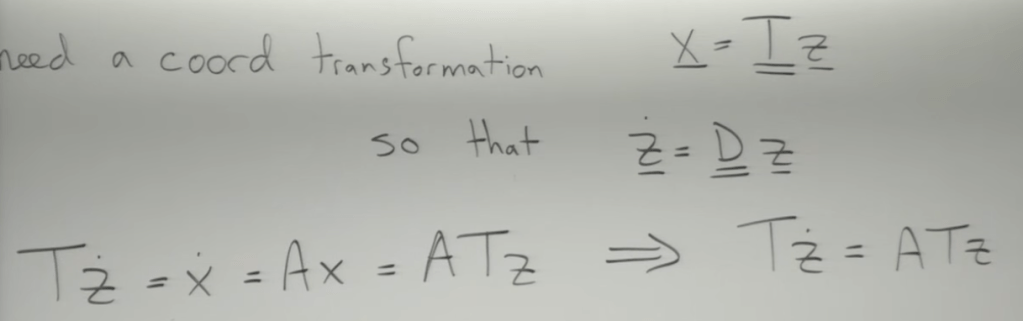
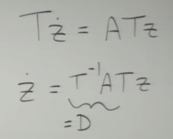
then we got eigenvector matrix format

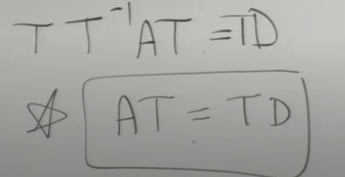
same as

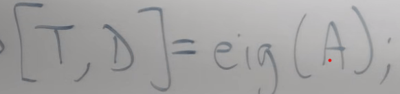
these math can all be realized in one line in matlab:

Setting stone for calculating e to the complex number exponential