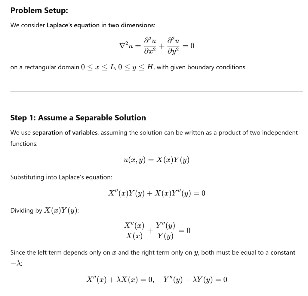
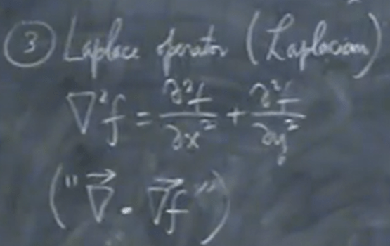
Background on heat equation one of the three canonical PDEs, so Laplace equation = 0, applying mechanical and numerical integral to solve (2D):

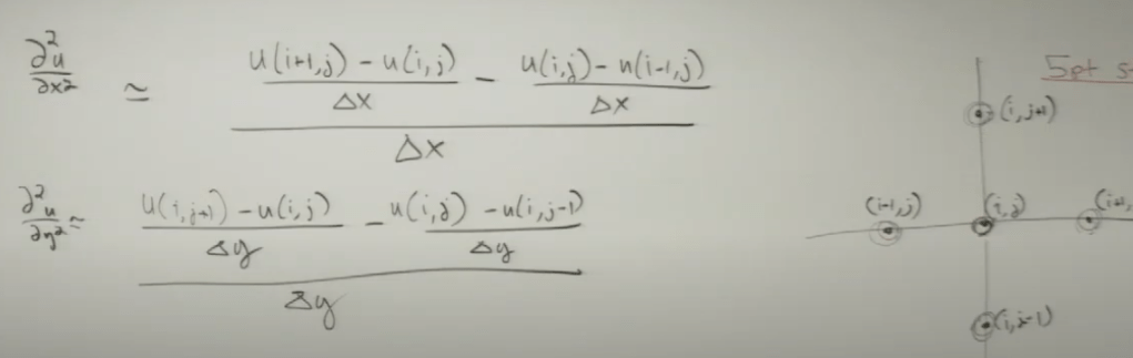
Next step to use 5-dot aid to reach to the equation for delta or gradients square:

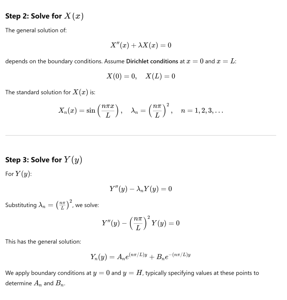
Another approach is to directly apply the equation from analytical function deduction:
in matlab
clear all, close all, clc
L = 100
H = 100;
u = zeros(L,H);
[X, Y] = meshgrid(1: 1: L, 1:1:H);
load seahawks.mat
colormap(CC);
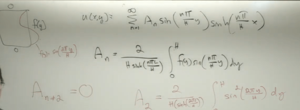
BC = sin(2*pi*(1:H)/H) ;
A2 = (2/(H*sih(2*pi*L/H)))*sum(BC.^2);
u = A2*sin(2*pi*Y/H)/*sinh(2*pi*X/H);
imagesc(u);
colorbar;
Adding on Nov 2021, high order partial derivate chapter by prof.Shifrin,
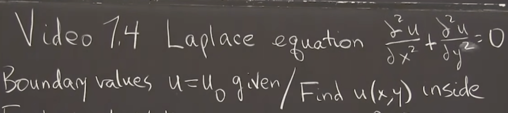
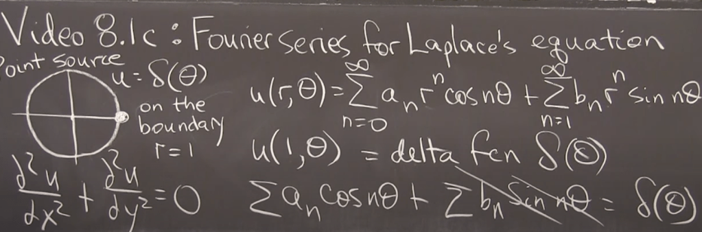
Enhance Laplace Equation by Prof. Gilbert Strang on Dec 19th, 2022:
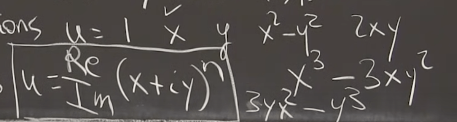
First, you can observe and try to find solution patterns:
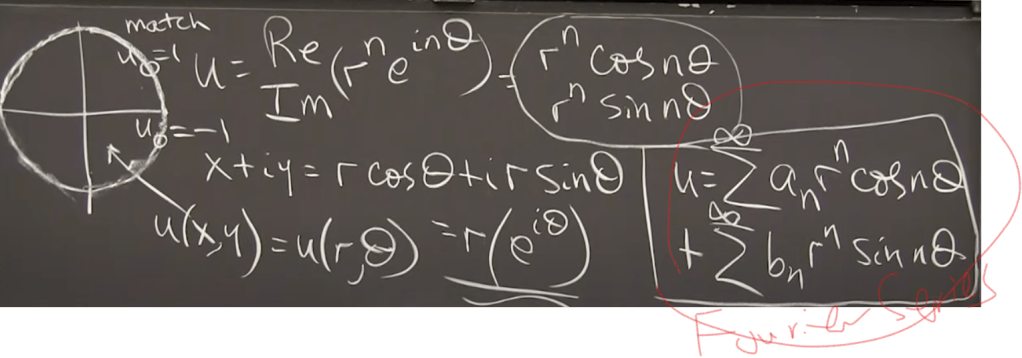
Then we’ll apply Fourier Series to solve the Laplace Equation, assuming there is a point source at r=1, theta=0
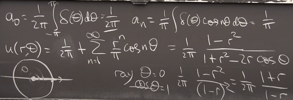
Explained step by step by AI