FFT is actually explained in the previous blog. The amazing thing is that now I can understand both audio and video files are fundamental same as they are both frequency files, one is frequency detected by ears the other by eyes.

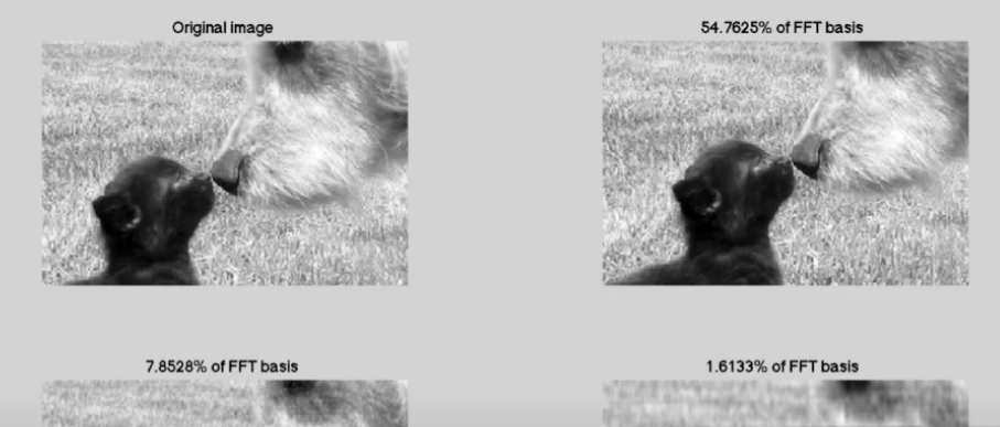
Note normal pictures can keep good quality throwing away 99%, however for those with hairs, furs, grass, FFT is not good at differentiating them, i.e. compression rate is much lower.

Compressive sensing might be a breakthrough with profound applications.

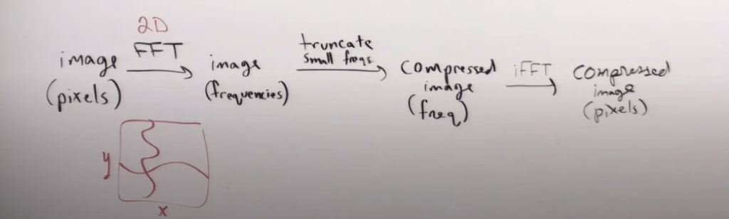
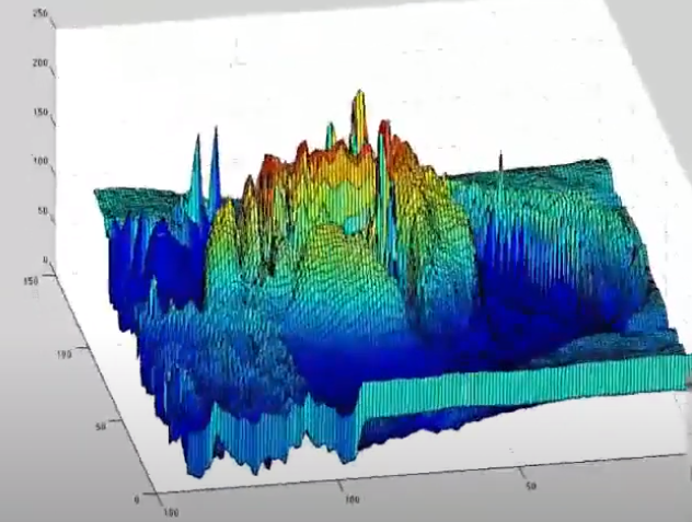
This frequency domain is composed of x and y axis, so we can picture it in below way

explanation by prof.Strang: link.

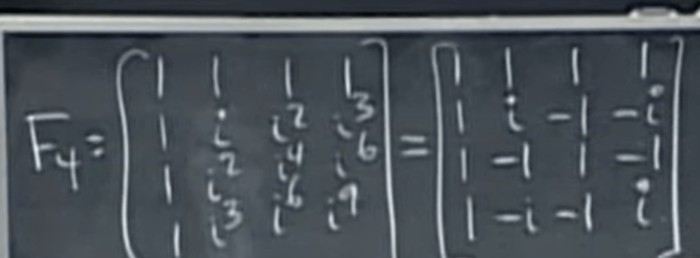
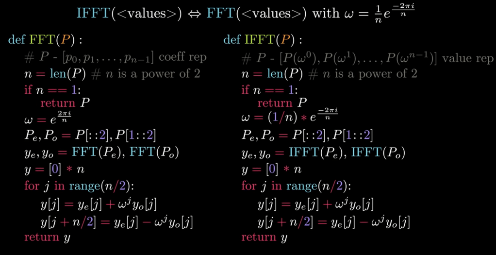
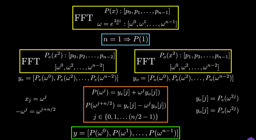
The FFT exploits symmetry in the Fourier matrix to reduce computation.

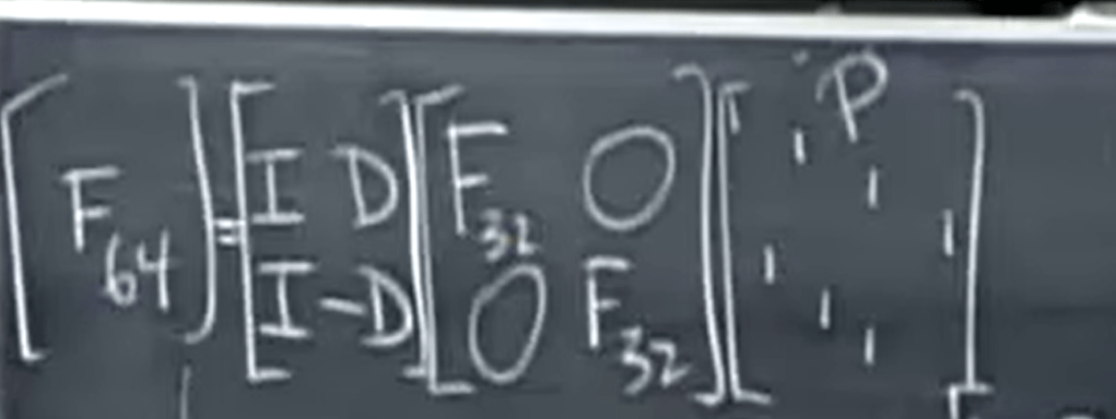
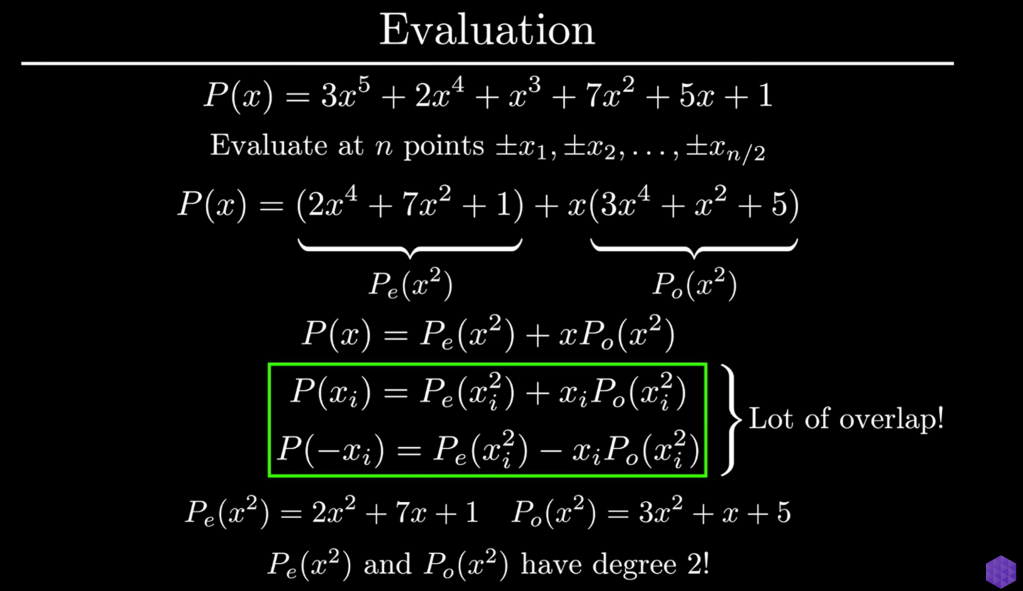
Smart mathematicians hundreds years ago was able to utilize FFT to do cumbersome polynomial multiplication, the key concepts are evaluation, interpolation (time domain to frequency domain), root of unity, recursive, domain expansion (from real Rn space to complex Cn space), pattern observation (odd and even both reducible to same and then can apply recursive algo). Big O n squared to Big O nlog(n). The ingenuity of reducing F64 to two F32 that was briefly stated by Dr.Strang is detailed here:

It’s mind-blowing beautiful MATH!

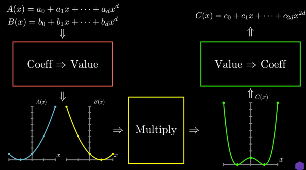
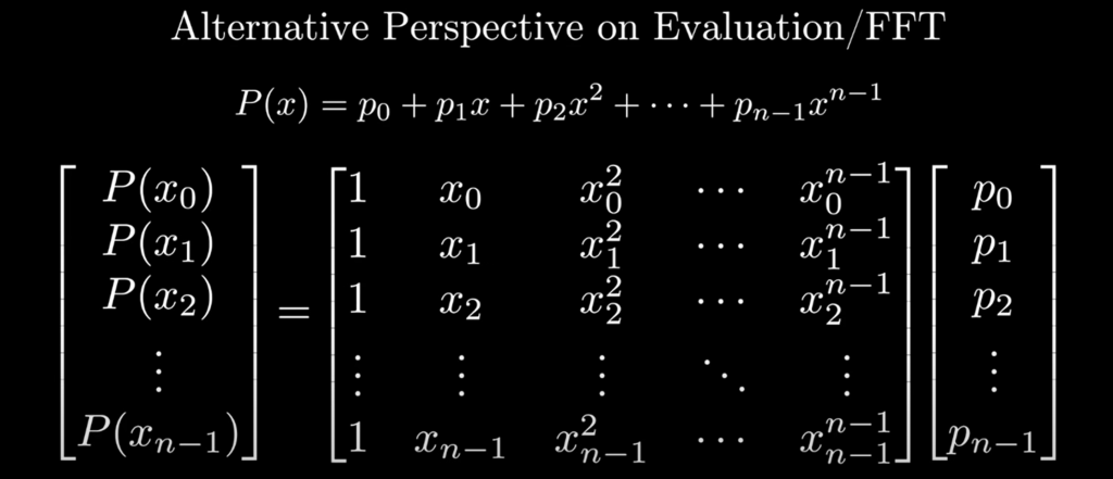
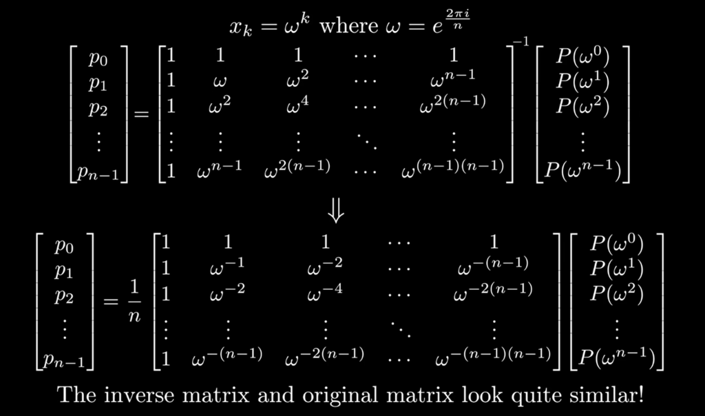
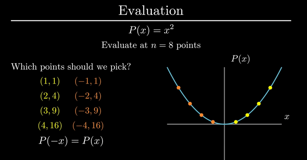
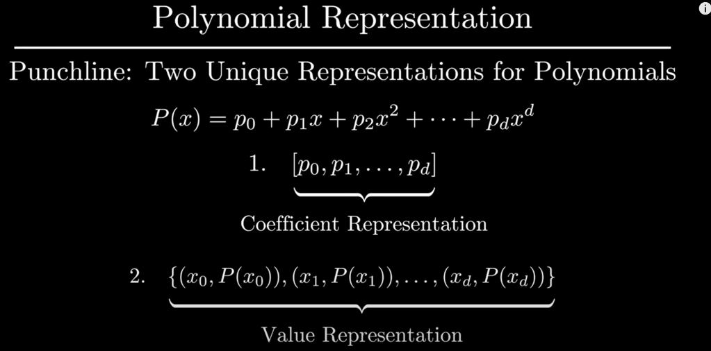
the crux explanation: any d degree polynomials can be represented by d+1 points. for any set of points there is a UNIQUE coefficient to represent the polynomial

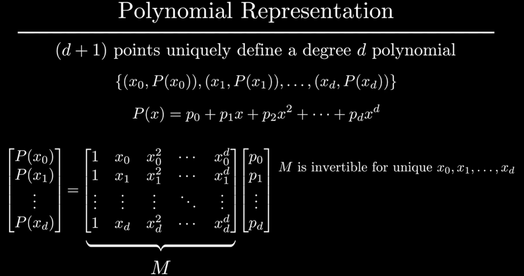
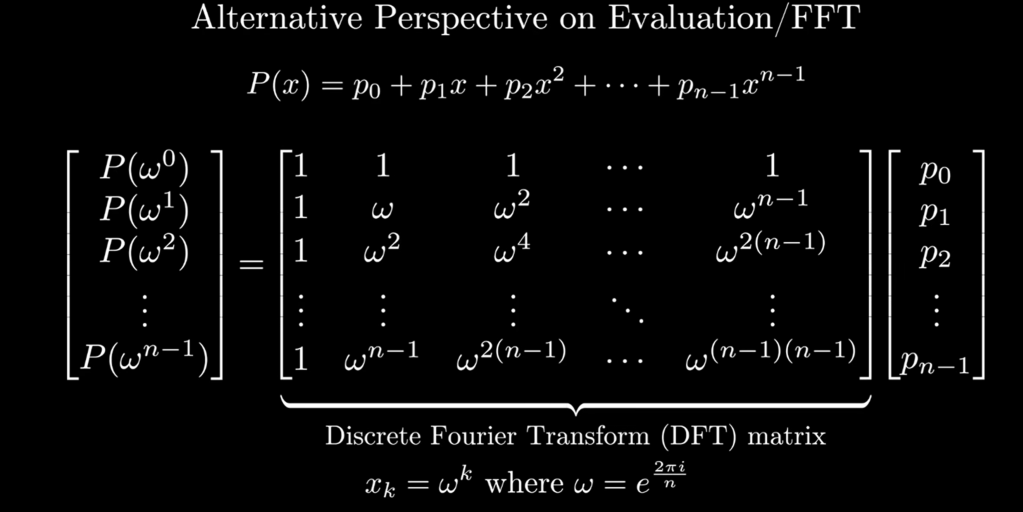
Here is the key connecting this polynomial computation to Fourier: the coefficient representation of polynomials is identical to Value representation. it’s like time domain FTed to frequency domain:

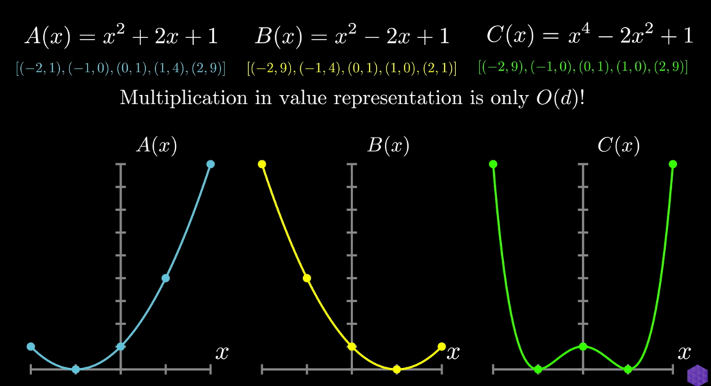
if polynomial is the the simple EVEN form:

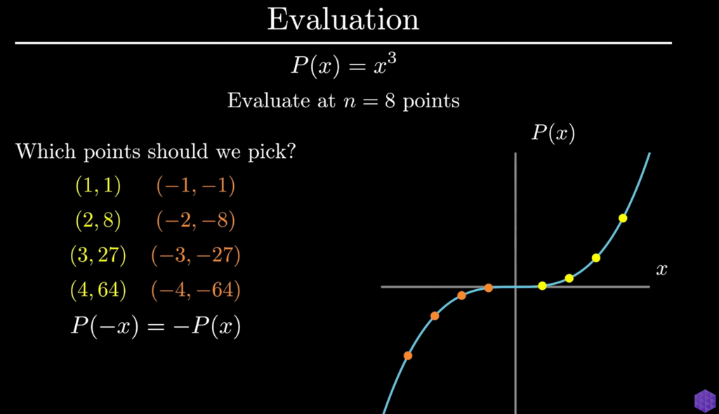
if the polynomial is the most simple ODD form

And this is something AI is still inadequate in educating while real master level mathematician can!