To use computers to calculate document similarity i.e. interpret documents as human beings do, semantic representations (i.e. embeddings) is the very first step.

LSA (latent semantic analysis) has been a primary approach in interpreting texts by dissecting documents into words matrix, and then applying SVD (single value decomposition) to identify the implied topic/concepts/meaning. The other recently developed approach is ML, where the very first step is Word2Vec.

I would explore the details between LSA and Word2Vec in this blog.

To explain LSA vectorization method, let’s use a toy example of 5 simple documents:

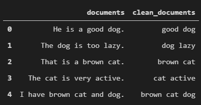
a1 = “He is a good dog.”a2 = “The dog is too lazy.”a3 = “That is a brown cat.”a4 = “The cat is very active.”a5 = “I have brown cat and dog.”df = pd.DataFrame()df[“documents”] = [a1,a2,a3,a4,a5]

After cleaning up the documents which include removing special characters, removing words with less than 3 letters, lowercase all words and removing all stop words (calling the package of nltk, from nltk.corpus import stopwords),

#remove words have letters less than 3
df['clean_documents'] = df['clean_documents'].fillna('').apply(lambda x: ' '.join([w for w in x.split() if len(w)>2]))
#lowercase all characters
df['clean_documents'] = df['clean_documents'].fillna('').apply(lambda x: x.lower())

import nltk
nltk.download('stopwords')
from nltk.corpus import stopwords
stop_words = stopwords.words('english')
# tokenization
tokenized_doc = df['clean_documents'].fillna('').apply(lambda x: x.split())
# remove stop-words
tokenized_doc = tokenized_doc.apply(lambda x: [item for item in x if item not in stop_words])
# de-tokenization
detokenized_doc = []
for i in range(len(df)):
    t = ' '.join(tokenized_doc[i])
    detokenized_doc.append(t)
df['clean_documents'] = detokenized_doc

get clean documents

Vectorization is realized by the following lines

from sklearn.feature_extraction.text import TfidfVectorizer
vectorizer = TfidfVectorizer(stop_words='english', smooth_idf=True)
X = vectorizer.fit_transform(df['clean_documents'])
X.shape #(5, 6)
dictionary = vectorizer.get_feature_names()
dictionary

The dictionary is

['active', 'brown', 'cat', 'dog', 'good', 'lazy']

Applying LSA,

from sklearn.decomposition import TruncatedSVD
# SVD represent documents and terms in vectors 
svd_model = TruncatedSVD(n_components=4, algorithm='randomized', n_iter=100, random_state=122)
lsa = svd_model.fit_transform(X)
lsa
#check the concepts/features
pd.options.display.float_format = '{:,.16f}'.format
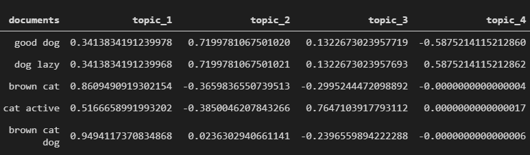
topic_encoded_df = pd.DataFrame(lsa, columns = ["topic_1", "topic_2", "topic_3", "topic_4"])
topic_encoded_df["documents"] = df['clean_documents']
display(topic_encoded_df[["documents", "topic_1", "topic_2","topic_3", "topic_4"]])

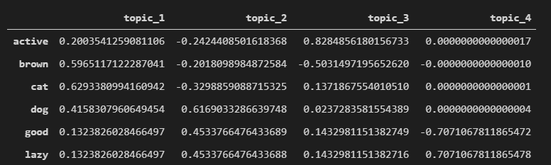
To view in an orthnormal perspective, meaning how each word is reflected in each topic/concepts

encoding_matrix = pd.DataFrame(svd_model.components_, index = ["topic_1","topic_2","topic_3", "topic_4"], columns = (dictionary)).T
encoding_matrix

One drawback of LSA is “in practice has some additional limitations. It makes no use of word order, thus of syntactic relations or logic, or of morphology. Remarkably, it manages to extract correct reflections of passage and word meanings quite well without
these aids, but it must still be suspected of resulting incompleteness or even errors.

LSA is powerful in analyzing a large set of data for topic surfacing, however, the more profound approach is “word embedding” or “word2vec”, and then apply machine learning algorithms such as SVM, Naive Bayers, Random Forest, RNN, LSTM bi-directional RNN etc. to accomplish complicated NLP tasks.

A very simple application is to compare documents similarity using Euclidean distance:

#simple distance of two documents
from sklearn.feature_extraction.text import CountVectorizer
from sklearn.metrics.pairwise import euclidean_distances

corpus = [
        'all my cats in a row',
        'when my cat sits down, she looks like a furby toy!',
        'the cat from outer space',
        'sunshine loves to sit like this for some reason'
        ]
vectorizer = CountVectorizer()
features = vectorizer.fit_transform(corpus).todense()
print(vectorizer.vocabulary_ )

for f in features:
    print(euclidean_distances(features[0], f) )

Vocabulary_ is {‘all’: 0, ‘my’: 11, ‘cats’: 2, ‘in’: 7, ‘row’: 14, ‘when’: 25, ‘cat’: 1, ‘sits’: 17, ‘down’: 3, ‘she’: 15, ‘looks’: 9, ‘like’: 8, ‘furby’: 6, ‘toy’: 24, ‘the’: 21, ‘from’: 5, ‘outer’: 12, ‘space’: 19, ‘sunshine’: 20, ‘loves’: 10, ‘to’: 23, ‘sit’: 16, ‘this’: 22, ‘for’: 4, ‘some’: 18, ‘reason’: 13}

Features is

matrix([[1, 0, 1, 0, 0, 0, 0, 1, 0, 0, 0, 1, 0, 0, 1, 0, 0, 0, 0, 0, 0, 0, 0, 0, 0, 0],
        [0, 1, 0, 1, 0, 0, 1, 0, 1, 1, 0, 1, 0, 0, 0, 1, 0, 1, 0, 0, 0, 0, 0, 0, 1, 1],
        [0, 1, 0, 0, 0, 1, 0, 0, 0, 0, 0, 0, 1, 0, 0, 0, 0, 0, 0, 1, 0, 1, 0, 0, 0, 0],
        [0, 0, 0, 0, 1, 0, 0, 0, 1, 0, 1, 0, 0, 1, 0, 0, 1, 0, 1, 0, 1, 0, 1, 1, 0, 0]], dtype=int64)

The distance of three docs relative to the very first one is

for f in features:…[[0.]] [[3.60555128]] [[3.16227766]] [[3.74165739]]

There are two most popular algorithms to create Word2Vec, one is Skip-Gram model and the other is Continuous Bag-of-Words model (CBOW). Skip-Gram method is to predict how likely it is for each word in the vocabulary being an input word’s nearby word. While CBOW is to predict how …

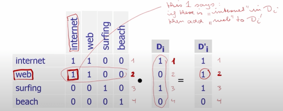
On Nov 16th, 2021, adding a systematic lecture from Prof.Bast on her course of IR(Information Retrieval) about LSI. Using an example of toy documents and terms as below, she leads to the concept of LSA intuitively.

A rigid dot product between this term-document matrix and the query Q vector will cause the issue that “internet surfing” is missed for query of “web surfing”, human can see it quickly but not this rudimentary form of math/machine reading.

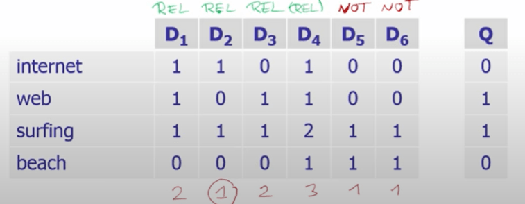
So we need to replace the two zeros with ones two as shown below

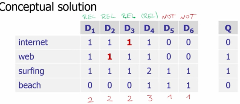
We want the machine to handle this automatically, so we want the machine to swap zeros to ones, so we identify the old matrix can be reduced to lower-rank base space B, composed of two underlying basic vector B1 and B2 as shown below.

And here is the concept of “matrix factorization” where we come up with the two base vectors B1 and B2 standing for each underlying concept. The new Doc vector with apostrophe are representation of the original document D in the lower-rank concept space of B. Matrix factorized.

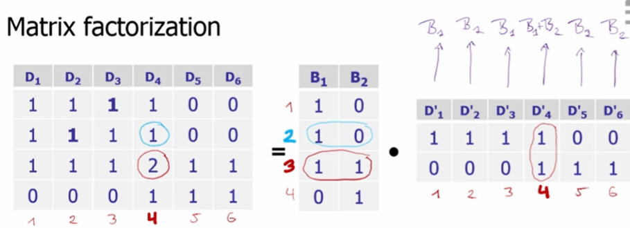
So to get the lower-rank base space B, which is shown as A’ in below screenshot, we resort to math, more specifically the math of distance calculation for similarity calculation.

The math trick to find A’ is SVD – single value decomposition. So what is SVD,

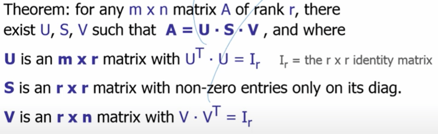
We can see this math “manipulation” does the realize the effect of human swapping zeros to ones as shown

How does SVD do so? Premised on basic knowledge on EVD, eigen value decomposition, we have

Gap here, needs to be expanded later.

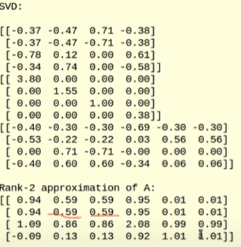
Anyway, now we use math to find the approximation of original A

There is an issue instantly pops out, the new truncated A’ is a dense (previous zero spaces are all filed up with values) matrix, the computation still can go hairy.

^To perceive it further, we can make the square matrix T^k as

So as long as internet shown up in Di not web, according to the T^k, a value of 1 will still be assigned … In essence, theis A dot At makes it possible to compute variance of two matrix(same) and figure our relationship between words.

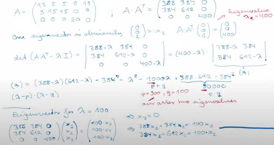
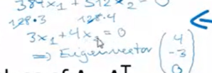
Let’s do a manual computation of a matrix A to find u, s, v.