0. In 1990, Deerwester et al. [Indexing by latent semantic analysis. J Am Soc Inform Sci 1990; 41: 391-407] published a technique called latent semantic analysis (LSA) to analyze term-by-document matrices. Based on this, a series of linear algebraic reduction methods are developed including: the nonnegative matrix factorization [15], semidiscrete matrix decomposition [16], probabilistic latent semantic indexing [17], and latent Dirichlet allocation [18] algorithms.

1. Sweden paper Evaluating Random Forest and a Long Short-Term Memory in Classifying a Given Sentence as a Question or Non-Question by FREDRIK ANKARÄNG and FABIAN WALDNER from KTH. Random Forest versus LSTM neural network for the task of classifying if a sentence is a question or not. The data used is Swedish articles from a local newspaper. RF is able to handle noisy data and more simplistic even overall LSTM outperformed RF with a slight margin. Moreover, the paper also conduct “customer service can be automated using a chatbot and what features and functionality should be prioritized by management during such an implementation.

Random Forest was originally proposed by Ho [4] in 1996 to address the tendencies of many decision tree based models to overfit. LSTM is a RNN contain a loop, where an input It1 is fed back to the network again with a new input It, in the process altering the output value ht. In theory the RNN can evaluate new input based on previous input and thus can be said to have a memory.

The data contained approximately 400,000 chat messages. The data mainly contained conversations between the users and customer service employees, as well as some automatically generated messages by the company’s chatbot. After cleaning, there are 13,758 sentences for classification.

This paper is practical in directing how companies implement chatbots.

2. Sparse Latent Semantic Analysis by Carnegie Mellon student and NEC Labs America, Princeton, NJ Xi Chen (1) Yanjun Qi(2) Bing Bai(2) Qihang Li(1) Jaime Carbonell. It seems to be published in 2004.

Sparse projection matrix via the ℓ1 regularization. Compared to the traditional LSA, Sparse LSA selects only a small number of relevant words for each topic and hence provides a compact
representation of topic-word relationships. Moreover, Sparse LSA is computationally very efficient with much less memory usage for storing the projection. It provides a pseudo probability distribution of each word given the topic, similar to Latent Dirichlet Allocation (LDA) (D. Blei, A. Ng, and M. Jordan. Latent dirichlet allocation. Journal of Machine Learning Research, 3:993–1022, 2003).

So what is the Sparse LSA, first, they conducted optimization formulation of LSA:

We consider N documents, where each document lies in an M-dimensional feature space X , e.g. tf-idf [1] weights of the vocabulary with the normalization to unit length. We denote N documents by a matrix X = [X1,… ,XM] ∈ R
N×M, where Xj ∈ R N is the j-th feature vector for all the documents. For the dimension reduction purpose, we aim to derive a mapping that projects input feature space into a D-dimensional latent space where D is smaller than M. When dealing with text data, each latent dimension is also called as a hidden “topic”.

Motivated by the latent factor analysis [7], we assume that we have D uncorrelated latent variables U1,… ,UD, where each Ud ∈ R N has the unit length, i.e. kUdk2 = 1. Here k · k2 denotes the vector ℓ2-norm and let U = [U1,… ,UD] ∈ R
N×D. We also assume that each feature vector Xj can be represented as a linear expansion in latent variables U1,… ,UD:

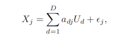
or simply X = UA + ǫ where A = [adj ] ∈ R D×M gives the mapping between the latent space and the input feature space and ǫ is the zero mean noise. Our goal is to compute the so-called projection matrix A.
We can achieve this by solving the following optimization problem which minimizes the rank-D
approximation error subject to the orthogonality constraint of U:

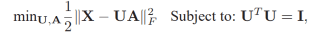
where k · kF denotes the matrix Frobenius norm and the constraint UT U = I guarantees that the
latent variables are uncorrelated with the unit length.

Next they applied the Sparse LSA on two widely adopted text classification corpora, 20 Newsgroups (20NG)
dataset 1 and RCV1 [10]. For the 20NG, we classify the postings from two newsgroups alt.tatheism and talk.religion.misc using the tf-idf of the vocabulary as features. For RCV1, we remove the words appearing fewer than 10 times and standard stopwords; pre-process the data according to [2] 2 ; and convert it into a 53 classes classification task.

Here is the comparison of their LSA and LDA in picking out the top 7 topics:

3. An Introduction to Latent Semantic Analysis by Department of Psychology University of Colorado at Boulder et al by Peter Foltz, Walter Kintsch, Thomas Landauer in 1998. It’s very interesting line “One might consider LSA’s maximal knowledge of the world to be analogous to a well-read nun’s knowledge of sex, a level of knowledge often deems a sufficient basis for advising the young.”

LSA has some additional limitations. It makes no use of word order, thus of syntactic relations or logic, or of morphology. Remarkably, it manages to extract correct reflections of passage and word meanings quite well without
these aids, but it must still be suspected of resulting incompleteness or likely error on some occasions.

4. Semantic Similarity of Short Texts University of Ottawa School of Information Tech. and Eng, authored by Aminul Islam and Diana Inkpen and published in 2014. Lots of papers are about documents analysis, this paper focuses on computing the similarity between two sentence or between two short paragraphs. There are existing methods: a). vector-based document model mothod: represent a document as a word vector and then queries are matched to similar documents via a similarity metric; b). corpus-based similarity: LSA (The dimension of the word by context matrix is limited to several hundreds because of the computational limit of Singular Value Decomposition (SVD). As a result the vector is fixed and the representation of a short text is very sparse.) and Hyperspace Analogues to Lanugage (HAL); c). hybrid use both corpus-based and knowledge-based measures; d). Another hybrid proposed by Li et al dynamically forms a joint word set only using all the distinct words in the pairs of sentences; e). Feature-based method try to represent a sentence using a set of predefined features.

This article proposed a method combining both semantic similarity and string similarity. misspelling tends to inadequatly treated by semantic similarity, so string similarity is necessary where longest common subsequence (LCS) is used so that it takes into account of the length of both the shorter and the longer string.

On the other hand, PMI-IR [38] is a simple method for computing corpus-based similarity of words which uses Pointwise Mutual Information. Then the detail of six steps in calculating. The emphasize the main upside of this method is less complexity and fast running speed due to avoidance of using WordNet or multiple corpus-based methods. by the way, WordNet is a lexical dataabase of semantic relations between words.

5. Turkish paper Using latent semantic analysis for automated keyword extraction from large document corpora in 2016. The goal is “automated keyword extractors”, one always can use curator based approach, but then data size grow astronomically, it is impossible, biomedical term extraction program is Metamap, a domain-specific knowledge base, an initiative launched and maintained by the National Library of Medicine. Then the authors did the Comparison of the Tf-idf, LSA, and Metamap keyword extraction methods using the ROC curve.

From above ROC curve, the Tf-idf thresholding method outperformed both variants of the LSA-based method and the Metamap method. Tf-idf used external information as it computed the weights using the complete set of documents. Using global information about the whole corpus gives the Tf-idf method a clear advantage.

The main advantage of our proposed method over Tf-idf is the mere utilization of the term weights of a single document at hand, whereas Tf-idf needs the knowledge of the whole document set in order to compute the inverse document frequency.

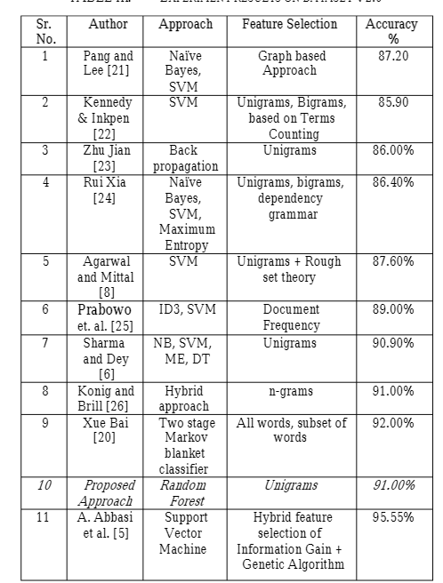
2020 paper by Indian A Novel Random Forest Implementation of Sentiment Analysis. The review portion the authors explained the reason for this study is to apply RF so to compare commonly used SVM with the following steps: download data from github, then exploration the data via visualization; data cleaning; TF-DF is used for creating features from text. It achieved f1 score of 0.66354

2014 paper by Indian again Sentiment Mining of Movie Reviews using Random Forest with Tuned Hyperparameters. Information gain and gain ratio are two methods to reduce features. Information gain is based on classified class, Gain Ratio contributes all features be normalized before classifying the document. RF classifier provides two types of randomness, first is with respect to data and second is with respect to features. Random Forest classifier uses the concept of Bagging and Bootstrapping. How RF works?

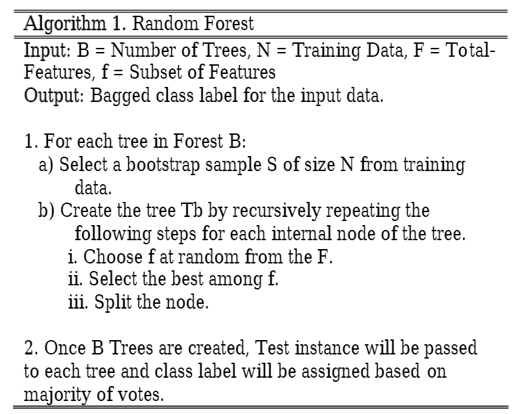
hyperparameters include number of tress to construct for the decision forest, number of features to select at random and depth of each tree. Movie Review Dataset V1.0 which consist of 1400 movie review out of which 700 reviews are positive and 700 reviews are negative. Second dataset consist of total 2000 Movie reviews and 1000 of which are positive and 1000 of which are negative.

dataset 2.0