Will follow the outlines as the following:

Advanced Mathematical Methods for Scientists and Engineers I
Asymptotic Methods and Perturbation Theory

The very first class on perturbation theory is very fascinating however, I need to revert to the basic of DE at Khan Academy again to be able to progress. So the following to follow through this video by Sal again.

Here are the summary of the important concepts and skills.

First, gradient of a scaler field (it forms a vector field), it can be interpreted as an operator that performs derivatives on each dimension.

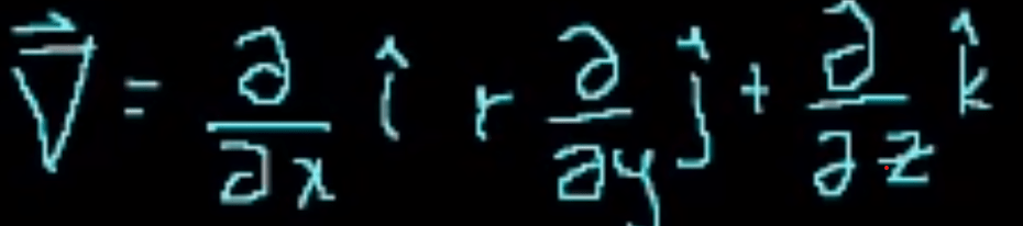
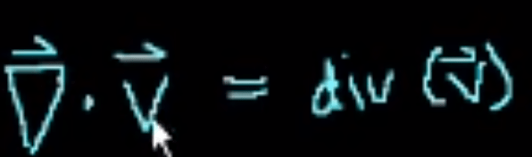
Second, Divergence of a vector at x and y (could be more dimensions), it reverse the previous process – from scaler to vector, here given a vector, it returns a scalar value. The computation is delta . vector.

Third, Curl of a vector, comparatively to div, curl measure the the torque force in the vector field.

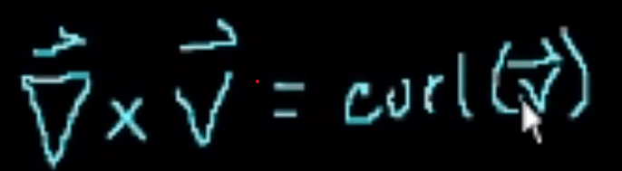
Here is a concrete example to perform curl computation

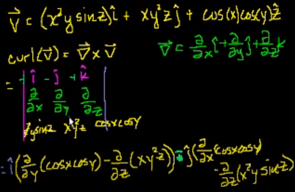
The question I ask is if Curl a scalar or vector? “In vector calculus, the curl is a vector operator that describes the infinitesimal circulation of a vector field in three-dimensional Euclidean space. The curl can be a scalar value after taking the cross product computation. But it also can be another form of vector, for example

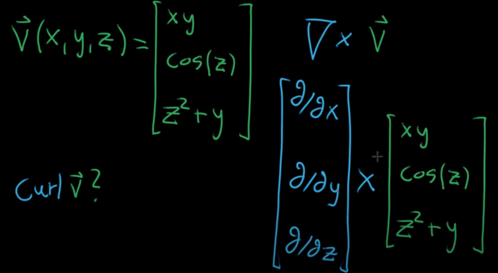
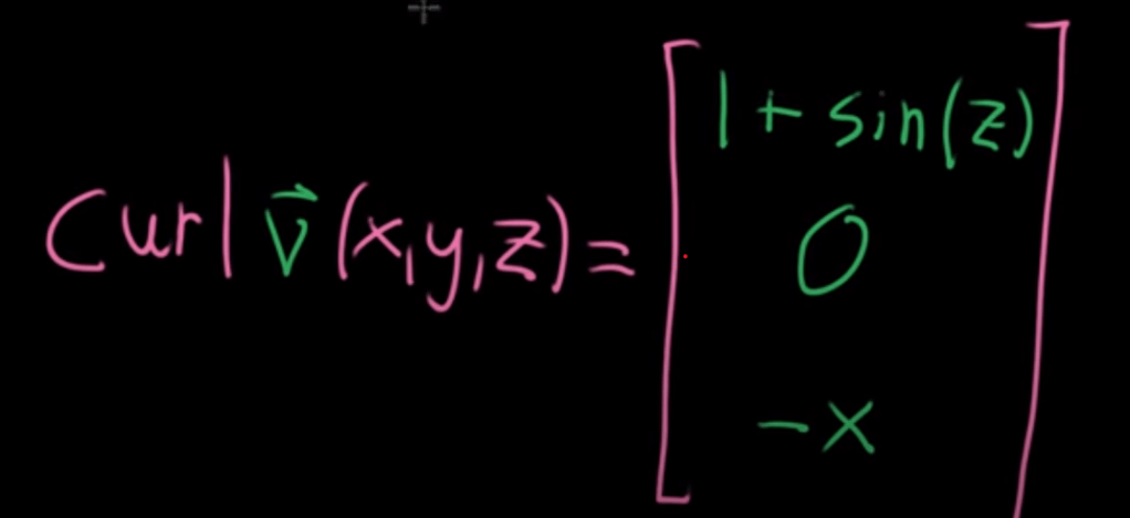
The final result is

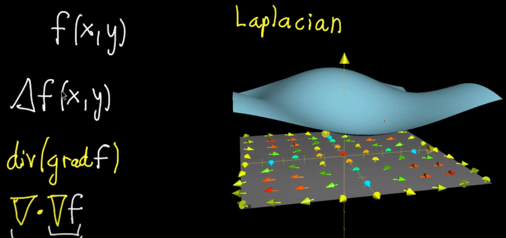
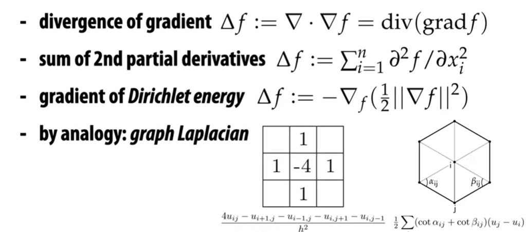
Fourth, Laplacian computation is defined as taking in a function composed of two scalar x and y, first take the gradient of f, which is a vector, then take the divergence of this vector (dot product) to get a scalar value. It’s like the second derivative in the sense that it denotes the speed of change, hence hints if the position is a minimum or maximum.

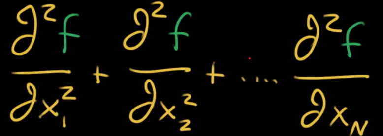
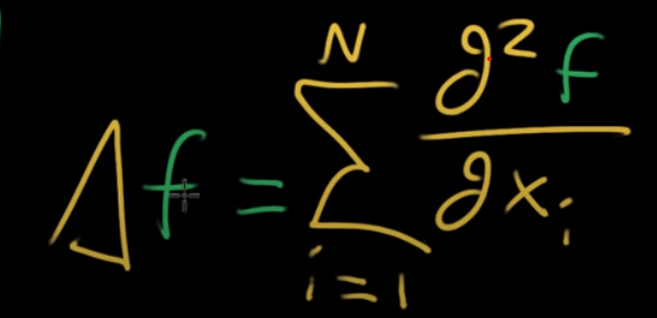
Laplacian formula can be written as the following when there are a lot more dimensions

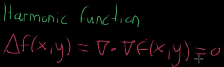
When the Laplacian value is 0, we call it harmonic function

Differentiate the concept between Laplacian and Hessian.

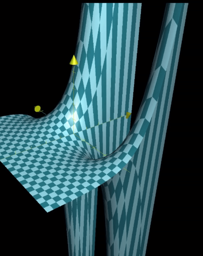
In two dimensional plane (x, y) it’s easy deduce the function is a straight line however in multi-dimensional venue, where Laplacian is used to compute minimum and maximum, there is a caveat such as the saddle function below, where the harmonic point has the feature of both minimum and maximum on respective axis/dimension.

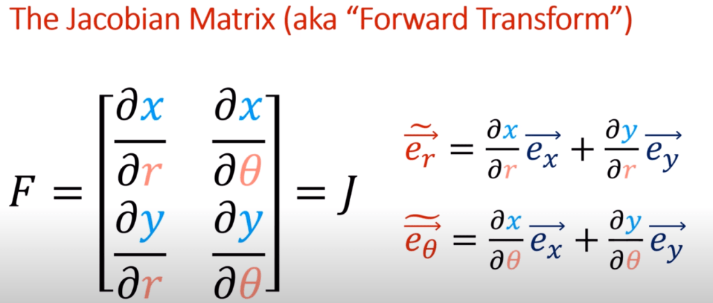
Fifth, Jacobian matrix, it is meant to tackle wavy/non-linear function on specific point by zooming in to transform non-linear to linear approximation.

Then we can compute the Jacobean determinant. It is said the major usage of Jacobean Matrix is to analyze the small signal stability of the system.

This concept of Jacobian Matrix has great meaning in learning Tensor, in forming forward transform to convert vector basis, the partial derivative formed matrix is named Jacobian matrix.

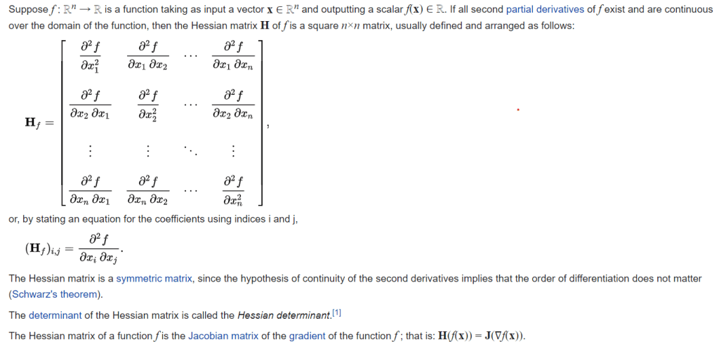
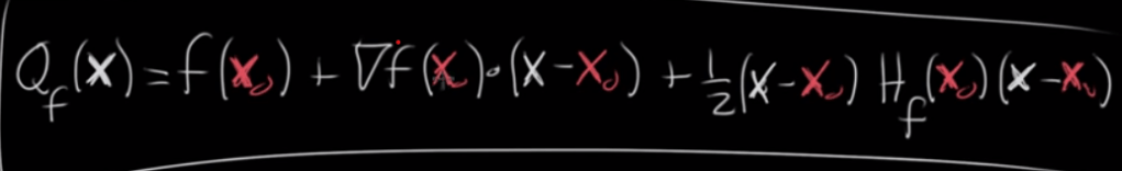
Sixth, Hessian matrices are used in large-scale optimization problems, providing the coefficient of the quadratic term of a local Taylor expansion of a function. That is

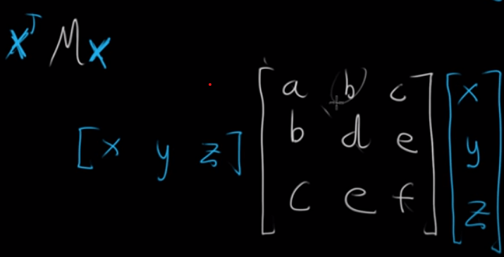
Why mathematicians love matrix format, it’s succinct and easy to handle more complex problems. For example, to Expressing a quadratic form with a matrix, if the form is ax + by + cz, it can be written as vector [a, b, c] dot vector [x, y, z] or V dot X; it is superb in quadratic forms

if there are three variables, one can get this

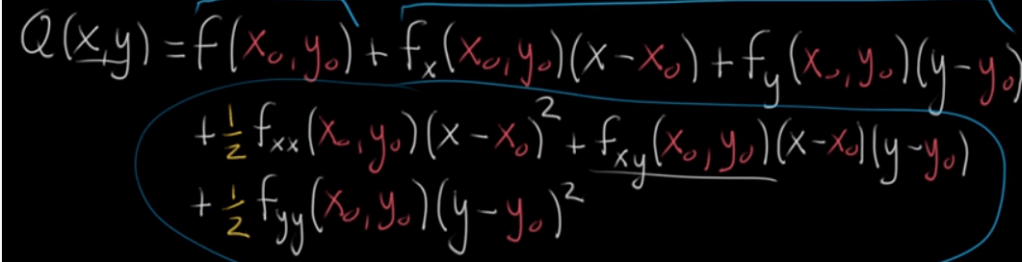
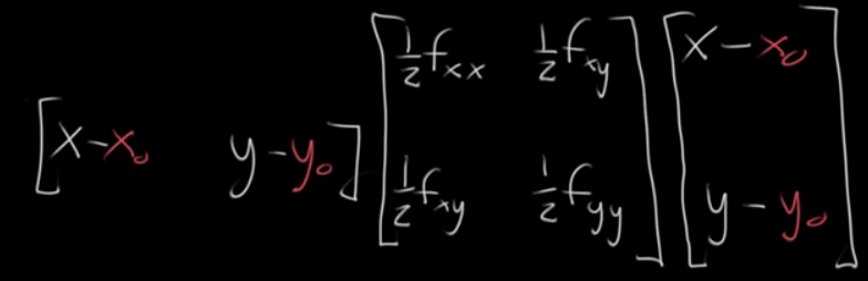
Now to apply this to approximate quadratic equation:

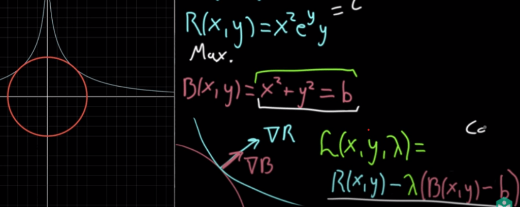
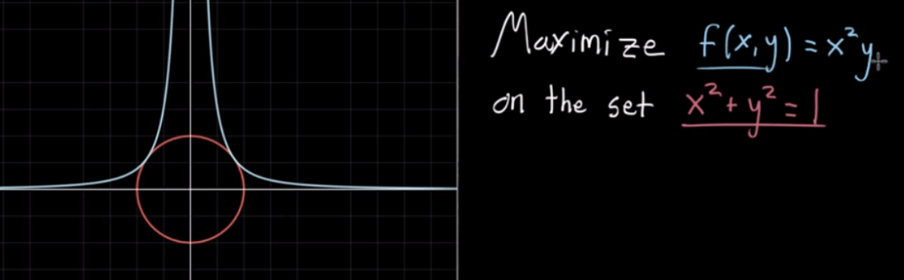
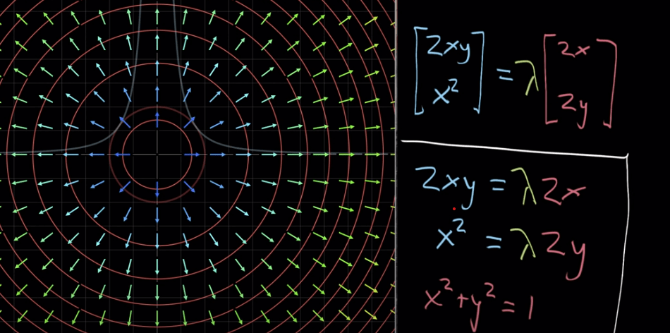
Seventh, Lagrange multiples in tackling Constrained Optimization problem for example to maximize the below function on the set of a circumference points. He cleverly uses the two perpendicular vector (gradient) to the tangency to plane. lambda is this Lagrange multiple that makes two equal other than the directions are identical.

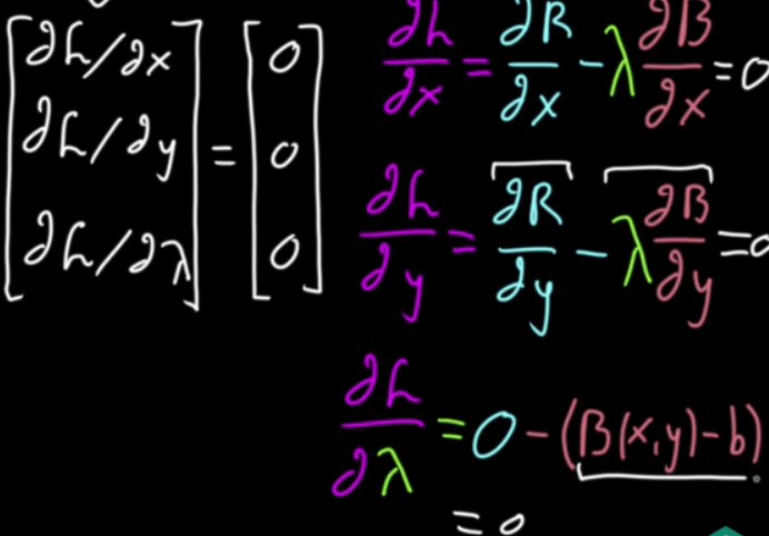
The seven and a halfth, derived from Lagrange multiples, is Lagrangian. It’s another clever way of encapsulating all needed math expressions: