All 2×2 orthogonal matrices can represent rotations if the QtQ=I is satisfied.

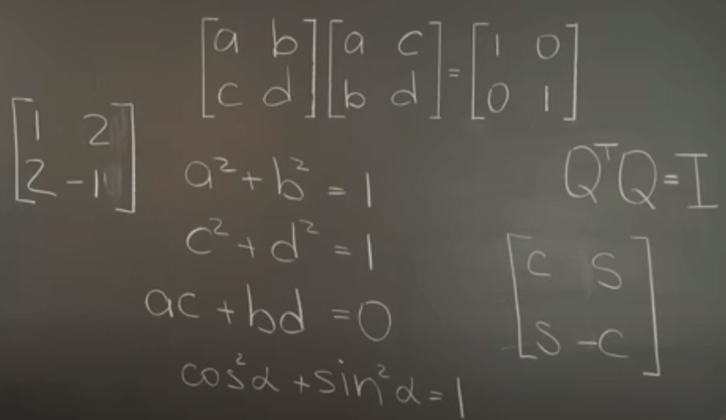
Note that CSS-C combination represent standard rotation, what about CS-SC, it can be written as CSS-C on a flip matrix[1,0; 0,-1], so it’s a flip then rotation.

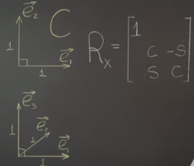
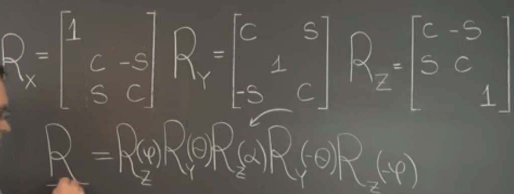
Moving on to try rotation in 3D space with respect to the Coordinate Axes, breaking it down to three scenarios where we hold x(e1), y(e2) and z(e3) axis fixed and then rotate the object, the formulas are

Before jumping to the essential concept of Euler Angles, first be very clear about the notion of longitude and latitude.

longitude 20° W, latitude 30° N. twisted certain angle. So the Euler Angles:

Next what about to Represent a Rotation with respect to an Arbitrary Axis?

3B1B talked lengthy about rotate and squish/squash is the essence of linear matrix transformation. Now with the basics of rotation in 3D gone through we visit this concept by Dr. Grinfeld.

Orthoscaling (aka Symmetric) Transformations has tremendous application in our life because the second derivative is an Orthoscaling transformation. There are these unique properties that 1). Orthoscaling Transformations Are (Sometimes) Represented by Symmetric Matrices, see proof below that if it’s orthonormal, then the equation holds. then S^t = S

2). Symmetric Matrices Have Orthogonal Eigenvectors. Proof is

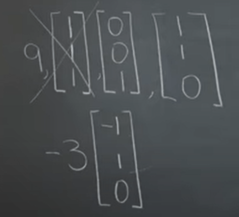
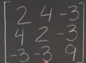
If we have symmetric matrix that have duplicated eigen value, such as

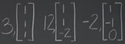
There are a plane as the eigen vector space, so we can subjectively choose the orthogonal vectors rather than one set that doesn’t satisfy orthogonal criteria:

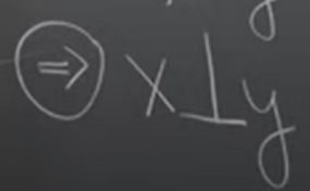
Note very important tip or skill to learn is that knowing one vector (2×2), then switching the position and adding a negative sign in front of either one, you get the orthogonal vector. It’s very useful in deducing eigen value vector pairs without going through cumbersome algorithm.

from MIT 18.06 review, symmetric matrixes are so important the feature is A = A^T. every symmetric matrix is a combination of perpendicular projection matrix.

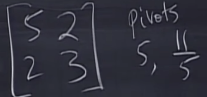
Then what is a positive definite symmetric matrix? Symmetrix matrix is good, then positive definite symmetric matrix is excellent. so the lambda and pivot are both positive. all subdeterminants are also positive.

Why do we take that much trouble understanding the symmetric matrices have these nice properties? We can use it to perform eigen value decomposition in a easy way, for example,

can be written in normal orthogonal format similarity transformation format:

Symmetric Matrices and the LDU Decomposition: After Gaussian elimination we can reach to LU as

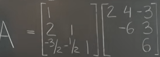
then single out the folds in middle diagonal, we can get LDU

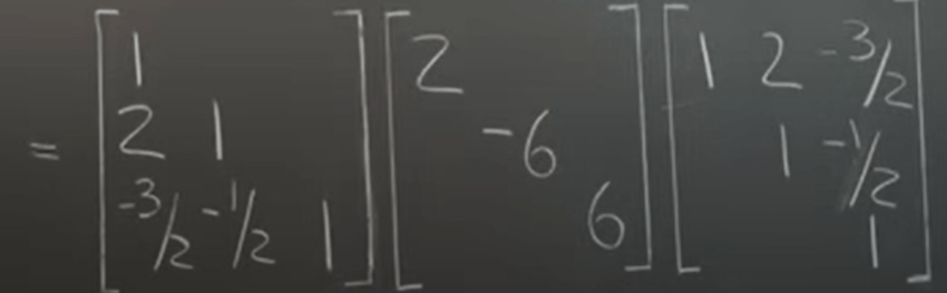
It looks quite similar in form to the eigen decomposition

What’s the difference? X is a normal matrix, but L is lower part matrix; lambda is eigen value, hard to compute while D is the pivot, easy to compute.

If the pivot is all positive figures, we can perform the Cholesky Decomposition, which is taking the square root of the pivot and equally distributed to each side, reducing the form to be L L^T.

Learning eigen value decomposition, LU decomposition, now Polar Decomposition – A Product of an Orthogonal and Symmetric Matrices. It has incredible value in actual world such as polynomial representation in Newton’s law, Fourier Transformation…

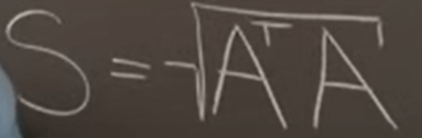
How to deduce? we need to leverage the beautiful properties of symmetric matrices, which is A^T A.

Following the construction thread

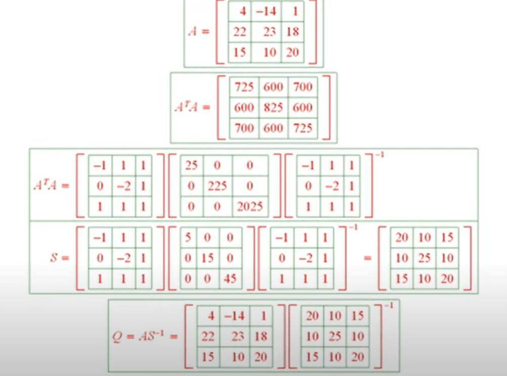
Note an important premise that the matrix has non-negative eigen values.

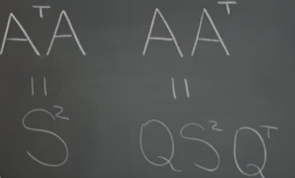
Next we can infer from below that these two are similarity transform, hence AᵀA and AAᵀ Have Identical Eigenvalues.

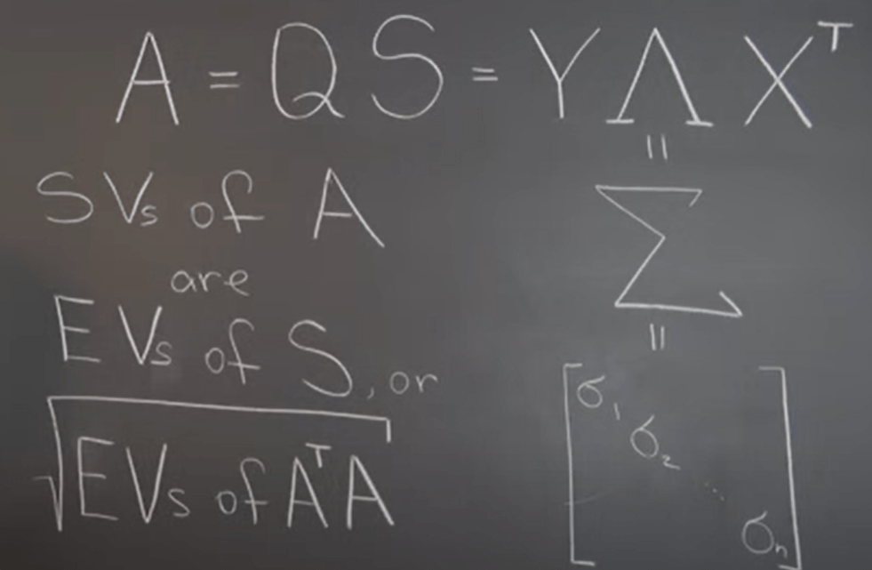
Lastly and foremost importantly, the Celebrated Singular Value Decomposition (SVD). It’s just one step away from A = QS composition elaborated above

Enhance on Dec 18th, 2022

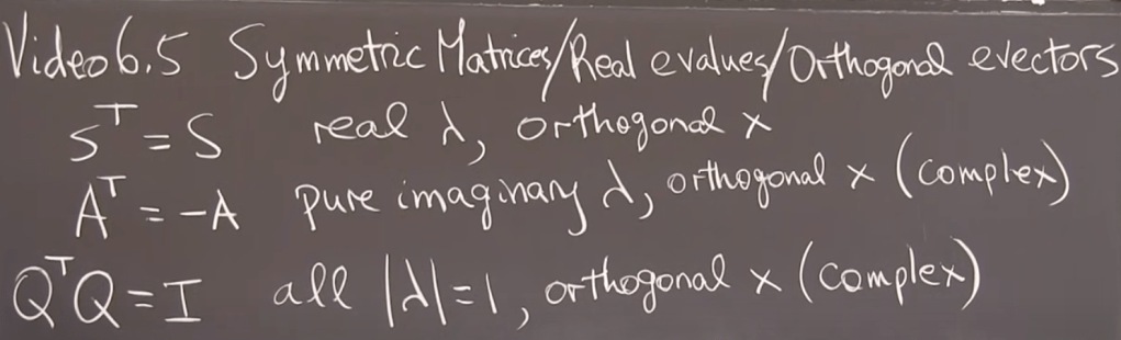
These different forms of matrix has the following geographic properties: first transpose is itself has real value as eigen values, the second has imaginary lambda(eigen values), and the third one’s eigen values stays on the circle, their eigen vectors are orthogonal.

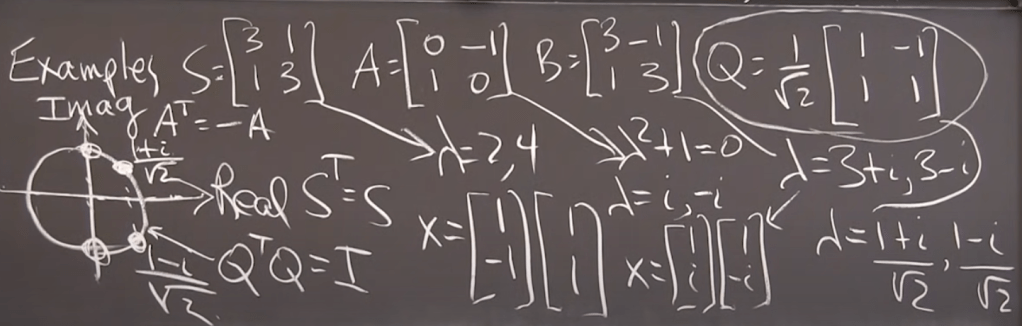
Note when there are complex components, always use conjugate part