Nobody knows who first defined but the definition of dot product or scalar product is given as

Based on this simple definition, we can deduce another vector p and q on a and b respsectively

Further, we get the widely used vector “decomposition” form
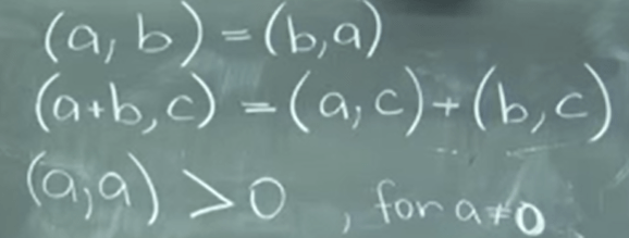
Now as a mathematician, being able to generalize abstractly, we identify the “dot product” itself is not a must, as long as the operation is communitive, distributive and self-operating is not zero(so the denominator is not zero), we can perform the same vector decomposition. We call it “inner product”. Expressed in math form it is
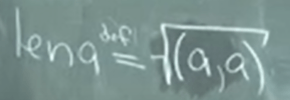
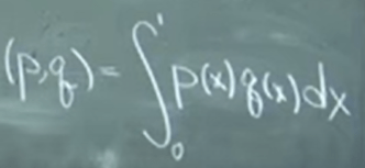
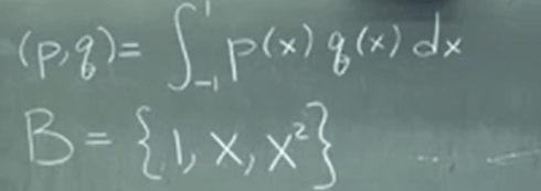
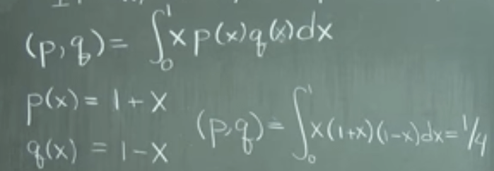
Now the most beautiful awesome part kicks in! Given this abstract definition and understanding we can define polynomial length. for example the below integral, taking in two functions(polynomials), spit out a scalar number, satisfies all inner product abstract axioms.
More example to get the concept sink in and grow
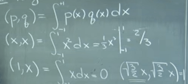
Note the last one square root of (3/2)x inner product is one, meaning it’s the unit length. Hence len(x) = square root of 2/3.
Similarly, (x, x^2) = 0 so these two components are orthogonal. Note what about (square root of x, square root of x)? this defies the very concept/definition of inner product, that the (a, a) is non zero positive, hence it’s not legit at all.
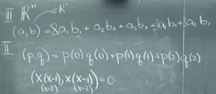
It’s really abstract to think through inner products esp. for polynomials, so for below (p, q), we reference top Rn outlay to get a sense if the arbitrarily decided inner product rule qualifies as inner product?
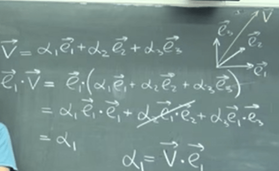
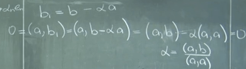
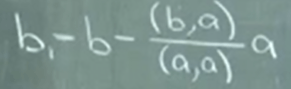
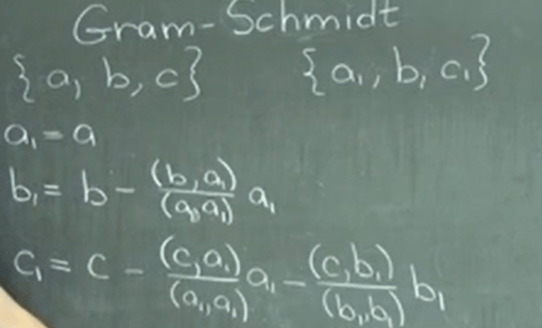
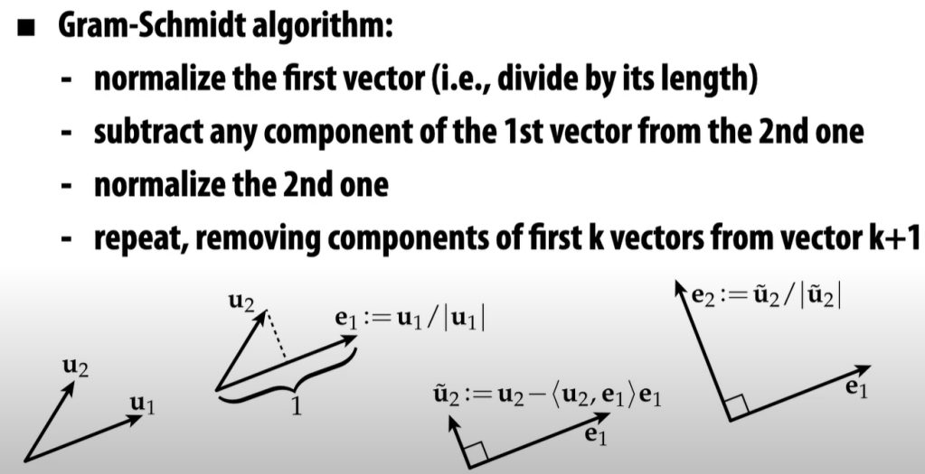
Orthogonal vectors are so important so we need to come up systematically an approach to find them. From the first diagram we got it geometrically, in the following we deduce in a rigorous manner to have the generic form.
Expanding to 3D space, orthogonal vectors are inferred as
This Gram-Schmidt algorithm is later elaborated when I go over “computer graphics” taught by Keenan Crane at CMU, and added here: “Gram-Schmidt algo is to normalize the first vector first then subtract any component of this 1st vector from the second one.”
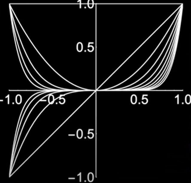
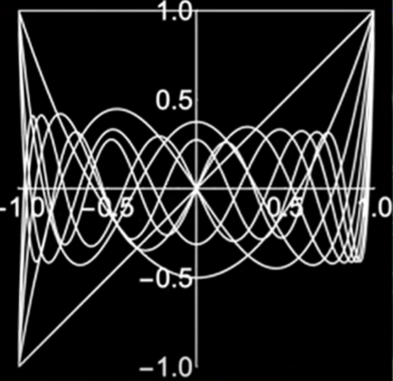
Why do we go through these painful seemingly trivial, we can apply it to polynomials to find corresponding orthogonal terms! for example in below integral function, we intuitively think set of B is the best basis, is it true? Are they orthogonal?
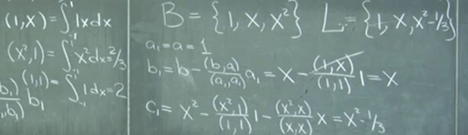
Put it into practice, Decomposition with Respect to Legendre Polynomials, it’s simply a mathematic computation.
Why the intuitive B = {1, x, x^2…) is a terrible basis while Legendre Polynomials are superior, it can be reflected on their geometric view
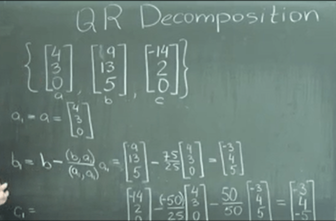
All above learning is to help solve pragmatic problems. Here we do QR composition using orthogonal method.
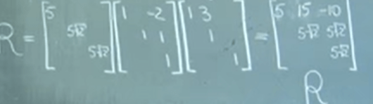
the following unorthogonal R3 can be computed into the a1, b1, c1, then we will compute orthonormal vectors.
Note the definition of inner product can vary but we choose the below one as the simplest form

now apply it (remember the matric conversion, since it’s acting on columns, we put identity matrix (operating object) to the right side and state it loudly to write down elementary matrix
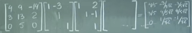
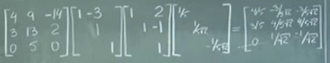
Now to get A = QR, reverse matrix need to be computed

Orthonormal columns means orthonormal rows – very important properties. Only orthogonal columns does not necessary have orthonormal rows unless they are normalized.
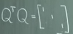
Determinant of the orthonormal matrix is +_1.
Inner product is so powerful here is an example to illustrate: the following integral is inner product, we can carry out the integral calculation which is simple,
we can also find the basis and only calculate 6 basis vector’s pair-wise gram or metric matrix, then we can recycle using this metric matrix over and over again for any such p and q integral problem
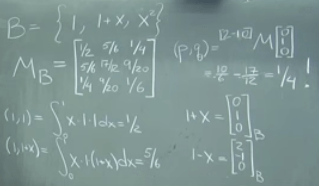
It is cumbersome at first but be powerful to carry more complex computation…
Added on Dec 2021, “QR decomposition, also known as a QR factorization or QU factorization, is a decomposition of a matrix A into a product A = QR of an orthogonal matrix Q and an upper triangular matrix R. QR decomposition is often used to solve the linear least squares problem and is the basis for a particular eigenvalue algorithm, the QR algorithm.”
Column space concept is consistent here with the QR process, it’s all about relationship between columns. It’s to identify linear relationship between columns and express in vector form.
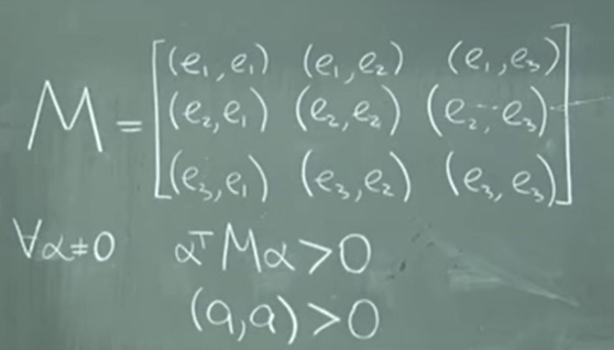
Least Square problems can all be reduced down to the QR decomposition in the sense that it is to calculate the minimum value of r=Ax-b, and we know rT dot r is the length. then it becomes an derivative matrix problem, where we need to convert to orthogonal matrix to solve. With an early harbinger of this tensor concept that a dot product (a, b) can always be essentially represented as

M is famously called “metrics”. In this context, components of M doesn’t necessary have to be orthogonal or orthonormal even it’s much easier to solve if they are.
Definition of tensor product is mentioned in identical particle in QM by Professor M.
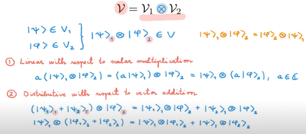
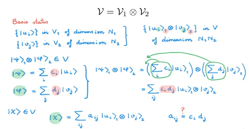
Entangled State is coined by Schrodinger by simply deducing from tensor product definition:

