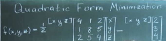
Moving to solving the real world problem, lot of them are minimization or optimization. Before we tackling complex problem such as
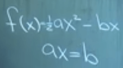
We start from the simplest form such as
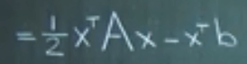
And for complex quadratic problems, they always reduce down to solve the same form
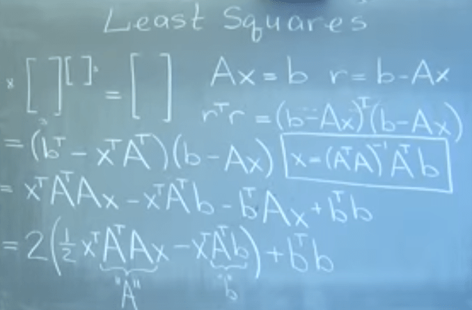
Now the real world problem where you have tons of rows but not as many columns(variables), the chances of solving it is near zero, so to minimize we suppose there is a length r that we can calculate that can be minimized
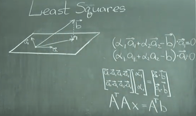
There is a geometric perspective to demonstrate the similar output:
We’ve been so used to least square since elementary school, this is the first it is fully explained how mathematicians came up with such a concept/solution:
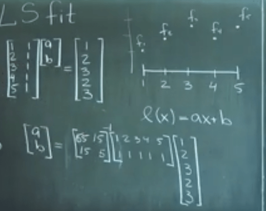
Often times in solving linear system equations like above under-constrained example, this concept of least square is manifested or realized by the optimization penalty method for exact, under-constrained or over-constrained situation(Explained in detail in Dr.Lum‘s lecture here), so basically if you are set to solve this three lines equation:
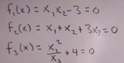
you can make it to be minimizing f0(x) = constant = 0 with constraints as below
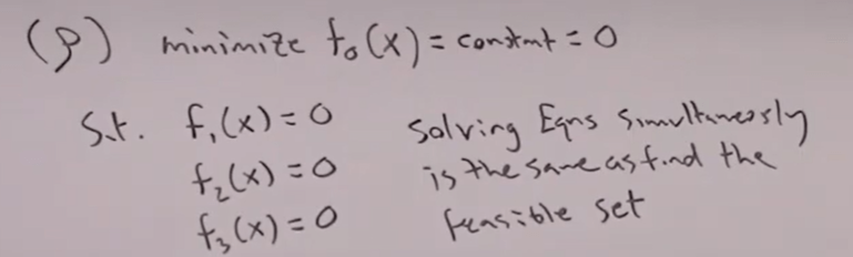
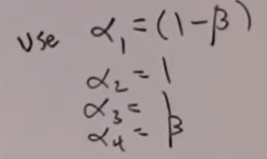
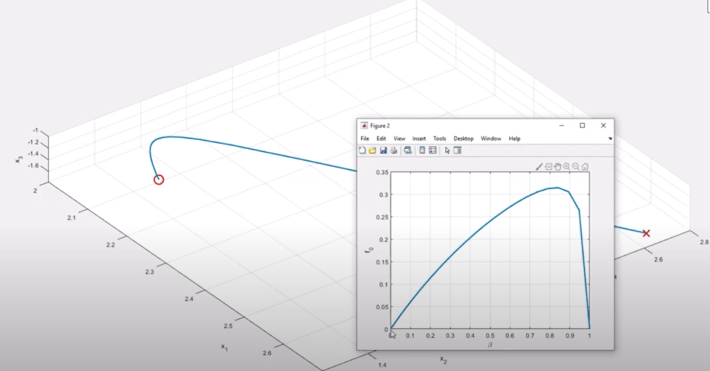
The setting of initial value as well as the alpha variable setting matters in searching for the optimal values. So if we add one more constraints making it unsolvable, but optimization still can be set to reach the “optimal” solution even it’s not possible to have a solution:
This is such a great math technique that we use to apply in control airplane dynamics.
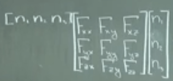
The Location of Minima and Maxima in Functions of Several Variables. To find this location, apply the idea of calculus – to find the derivative that is 0. So imagine there is a candle burning in the center of a room, you can draw an arbitrary line along the tip of candle and set a parameter alpha or time t to go through this line, the closer it is to the tip of flame, the higher the temperature scalar is. In the same vein, we can draw multiple lines naming them, x, y, z as below:
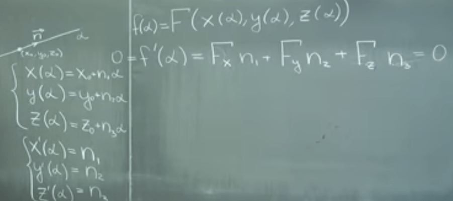
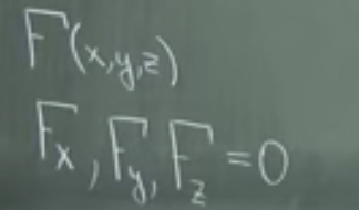
Conclusion is that on each dimension, F’s partial derivative to x, y, z must equal to zero respectively.
For this location to be the minimum, the second derivative has to be greater than 0, see
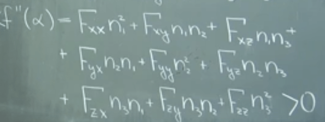
Written in matrix formula