PDF, according to wiki, probability density function (PDF), or density of a continuous random variable, is a function whose value at any given sample (or point) in the sample space (the set of possible values taken by the random variable) can be interpreted as providing a relative likelihood that the value of the random variable would equal that sample. Note not every probability distribution has a density function: the distributions of discrete random variables do not. A distribution has a density function if and only if its cumulative distribution function F(x) is absolutely continuous. In this case: F is almost everywhere differentiable, and its derivative can be used as probability density.

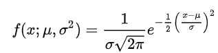
The normal distribution is parametrized in terms of the mean and the variance, denoted by mu and sigma respectively,

Then we need to explore Binominal distribution, Poisson distribution, Bernoulli distribution and Chi-square distribution.

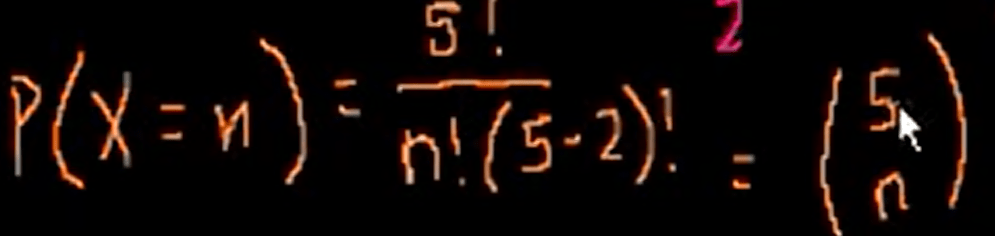
Use coin flipping as an example to illustrate the Binomial distribution, if in each round you flip 5 times and here we list out the probability of Variable X as to get zero head, one head… and 5 head, then draw the distribution graph:

The coefficient can be calculated as

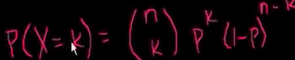
The expected value of bionominal distribution with a individual probability ad-hoc value p

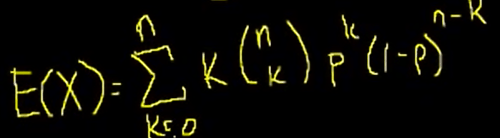
the math proving of above E(x) is majestic! can refer back to Sal’s video again.

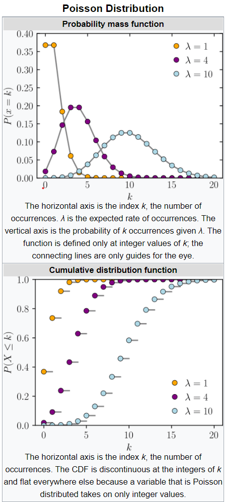
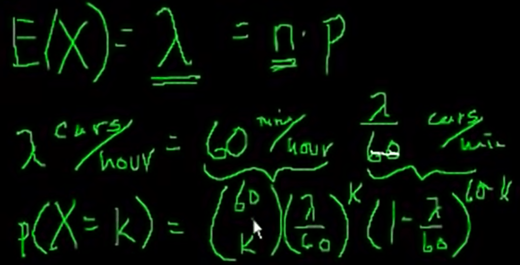
Poisson distribution is to describe event such as number of cars passing in an hour in an intersection.

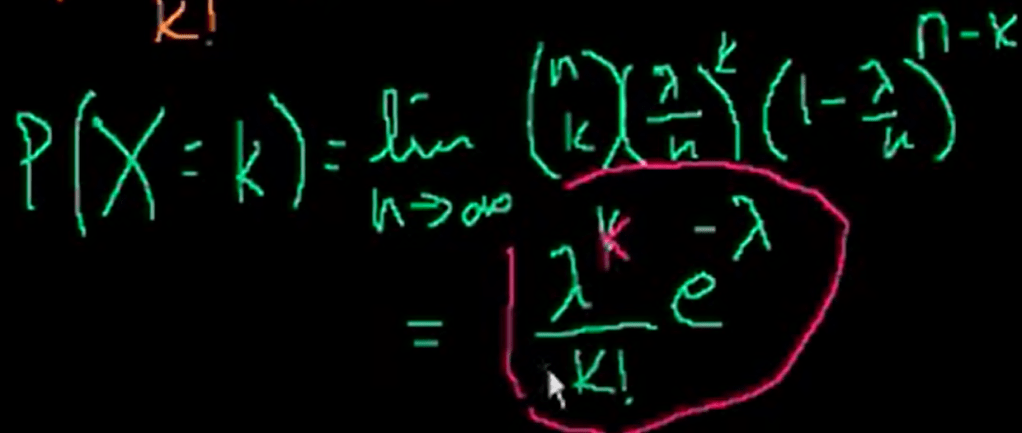
We can convert it to be a binominal problem by breaking the interval one hour here to infinite small number of trying/coin flipping.

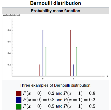
Bernoulli distribution is the discrete probability distribution of a random variable which takes the value 1 with probability p and the value 0 with probability q, q = 1-p. Less formally, it can be thought of as a model for the set of possible outcomes of any single experiment that asks a yes–no question. It’s easy to infer that E(x) = p and variance = p(1-p).

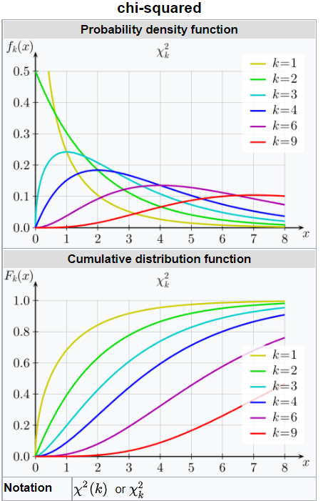
Chi-squared distribution (also chi-square or χ2-distribution) with k degrees of freedom is the distribution of a sum of the squares of k independent standard normal random variables. The chi-squared distribution is a special case of the gamma distribution and is one of the most widely used probability distributions in inferential statistics, notably in hypothesis testing and in construction of confidence intervals.

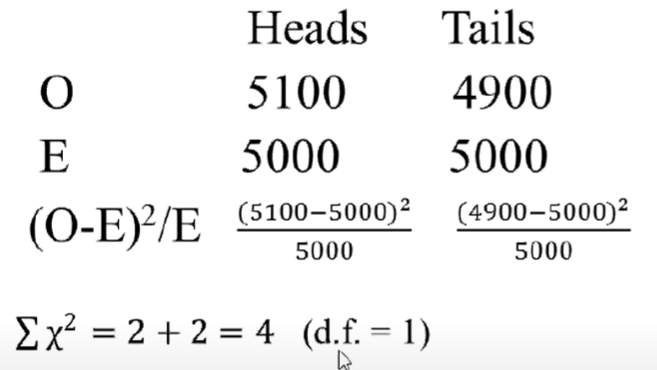
In college, we were told to apply Chi-square test for experiment results, but the teacher never made clarified why. Recently I found the Mathoma vedio giving an explanation in great detail, the title is Interpretation of (O-E)^2/E, however, it is still not perfectly clear.

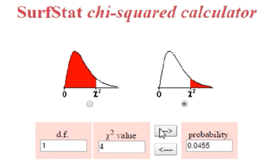
He basically uses flipping coin/binomial distribution, when the sample size is large enough, the binomial distribution is consistent to the normal distribution(see the first part of this blog). So we can perform Z-test and turn out the p = 0.0455, reject the null hypothesis.

What Mathoma demonstrated is that this result is exact as the Chi-square test

He also went forward to prove the sigma is identical in normal distribution and Chi-square test.

Touching on gamma distribution, a random variable X that is gamma-distributed with shape α and rate β is denoted

Chi-square test is used on contingency tables and more appropriate when the variable you want to test across different groups is categorical. It compares observed with expected counts. Both t test and ANOVA are used to compare continuous variables across groups.

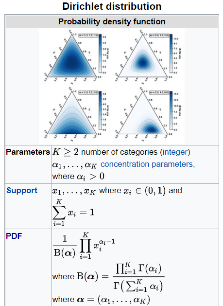
Lastly and most importantly for my research, Dirichlet distribution (after Peter Gustav Lejeune Dirichlet), often denoted Dir(alpha ), is a family of continuous multivariate probability distributions parameterized by a vector alpha of positive reals.