The ultimate purpose of learning PuLP is to apply it in finance especially investment optimization. So let’s first touch on the simple case and then would be able to go deeper.
From Ahershy, I borrow this case:
The objective is to Minimize risk while meeting Goals / Constraints:
-Minimum return at least 7.5%

-At least 50% of investment A rating

-At least 40% of investment immediately liquid

-max in savings and cd = $30,000
| Designation | Potential Investment | Expected Return | Rating | Risk | Liquidity | Saving&CD | Amt_Invested | |
|---|---|---|---|---|---|---|---|---|
| 0 | x1 | Savings Account | 0.040 | 1 | 0 | 1 | 1 | 1 |
| 1 | x2 | Certificate of Deposit | 0.052 | 1 | 0 | 0 | 1 | 1 |
| 2 | x3 | Atlantic Lighting | 0.071 | 0 | 25 | 1 | 0 | 1 |
| 3 | x4 | Arkansas REIT | 0.100 | 0 | 30 | 1 | 0 | 1 |
| 4 | x5 | Bedrock Insurance Annuity | 0.082 | 1 | 20 | 0 | 0 | 1 |
| 5 | x6 | Nocal Mining Bond | 0.065 | 0 | 15 | 0 | 0 | 1 |
| 6 | x7 | Minocomp Systems | 0.200 | 1 | 65 | 1 | 0 | 1 |
| 7 | x8 | Antony Hotels | 0.125 | 0 | 40 | 1 | 0 | 1 |
#simple in the sense that it only requires variable formed in dictionary not necessary the convoluted form as in Sudoku's
prob = LpProblem("Portfolio_Opt",LpMinimize)
prob
# Create a list of the inventment items
inv_items = list(df['Potential Investment'])
# Create a dictinary of risks for all inv items
risks = dict(zip(inv_items,df['Risk']))
# Create a dictionary of returns for all inv items
returns = dict(zip(inv_items,df['Expected Return']))
#Create dictionary for ratings of inv items
ratings = dict(zip(inv_items,df['Rating']))
# Create a dictionary for liquidity for all inv items
liquidity = dict(zip(inv_items,df['Liquidity']))
#Create a dictionary for savecd for inve items
savecd = dict(zip(inv_items,df['Saving&CD']))
#Create a dictionary for amt as being all 1's
amt = dict(zip(inv_items,df['Amt_Invested']))
risks
inv_vars = LpVariable.dicts("Potential Investment",inv_items,lowBound=0,cat='Continuous')
inv_vars
#inv_vars look like
# {'Savings Account': Potential_Investment_Savings_Account,
#  'Certificate of Deposit': Potential_Investment_Certificate_of_Deposit,
#  'Atlantic Lighting': Potential_Investment_Atlantic_Lighting,
#  'Arkansas REIT': Potential_Investment_Arkansas_REIT,
#  'Bedrock Insurance Annuity': Potential_Investment_Bedrock_Insurance_Annuity,
#  'Nocal Mining Bond': Potential_Investment_Nocal_Mining_Bond,
#  'Minocomp Systems': Potential_Investment_Minocomp_Systems,
#  'Antony Hotels': Potential_Investment_Antony_Hotels}

prob += lpSum([risks[i]*inv_vars[i] for i in inv_items])
prob

# amt
prob += lpSum([amt[f] * inv_vars[f] for f in inv_items]) == 100000, "Investments"
prob += lpSum([returns[f] * inv_vars[f] for f in inv_items]) >= 7500, "Returns"
prob += lpSum([ratings[f] * inv_vars[f] for f in inv_items]) >= 50000, "Ratings"
prob += lpSum([liquidity[f] * inv_vars[f] for f in inv_items]) >= 40000, "Liquidity"
prob += lpSum([savecd[f] * inv_vars[f] for f in inv_items]) <= 30000, "Save and CD"

prob.solve()
prob.writeLP("Portfolio_Opt.lp")
print("The optimal portfolio consists of\n"+"-"*110)
for v in prob.variables():
    if v.varValue>0:
        print(v.name, "=", v.varValue)

# The optimal portfolio consists of
# --------------------------------------------------------------------------------------------------------------
# Potential_Investment_Arkansas_REIT = 22666.667
# Potential_Investment_Bedrock_Insurance_Annuity = 47333.333
# Potential_Investment_Certificate_of_Deposit = 12666.667
# Potential_Investment_Savings_Account = 17333.333
Now to touch bit deeper in this kind of problem, let’s refer to the textbook case form mathworks. The bond portfolio has variation on yield and maturity:
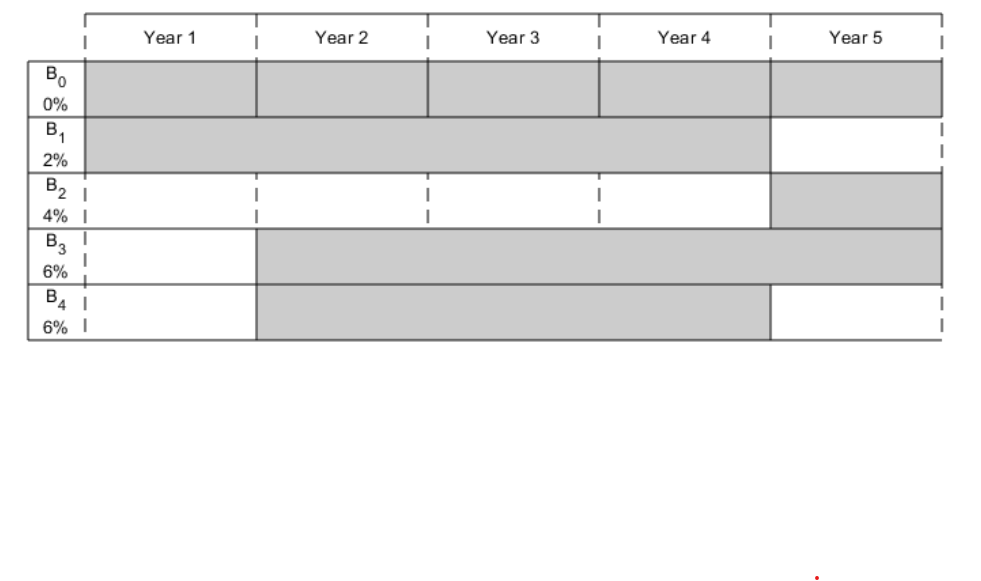
The rest is similar, constraints are:
invest no more than you have;
no borrowing
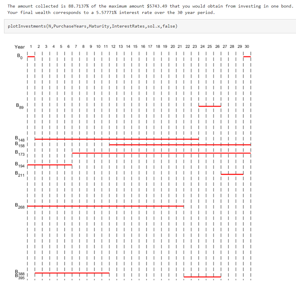
Then solve the problem. The beauty of this set up is that it can be generalized to much complex, bigger case, Create a model for a general version of the problem. Illustrate it using T = 30 years and 400 randomly generated bonds with interest rates from 1 to 6%. This setup results in a linear programming problem with 430 decision variables.