My goal is to figure out the code behind portfolio optimization commercialized by firms such as Axioma (now merged to Qantigo), given a good taste of how simple PuLP package can solve. The first dab is on MIT 6.0002 series lectured by senior professors, the other is a good book from Amazon – Pyomo — Optimization Modeling in Python, published by Springer, authored by Michael Bynum, Gabriel Hackbeil etc.
First, quick dive into the series Introduction to Computational Thinking and Data Science. These basic concepts worth revisiting. It was in the second course, the professor mentioned the notion of “dynamic programing”. Where memozation is applied:
# A memoized solution
def fib_2(n, memo):
    if memo[n] is not None:
        return memo[n]
    if n == 1 or n == 2:
        result = 1
    else:
        result = fib_2(n-1, memo) + fib_2(n-2, memo)
    memo[n] = result
    return result

def fib_memo(n):
    memo = [None] * (n + 1)
    return fib_2(n, memo)
The contents of the textbook Pyomo is laid out as such
Introduction: key pyomo features
PartI An Introduction to Pyomo: Mathematical Modeling and Optimization; Pyomo Overview, components; Scripting Custom Workflows; Interacting with Solvers;
PartII Advanced Topics: nonlinear programing with Pyomo (Rosenbrock problem..); Structured Modeling with Blocks; Performance, modeling construction and solver interfaces; Abstract Models and Their solutio;
PartIII Modeling Extensions: Generalized disjunctive programing (solve GDP model, Big-M transformation, Hull Transformation); Differential Algebraic Equations; Mathematical Programs with Equilibrium Constraints.
There free open sources (PuLP) as well as for-profit optimizer (Matlab, Gurobi Optimizer) in market.
I’d like to dive bit deeper on the code behind that realize risk minimization and return maximization in matlab, in it’s website details more info than Gurobi:
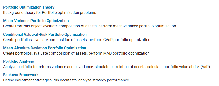
- Portfolio optimization theory is based on mean-variance portfolio optimization (see Markowitz [46], [47] at Portfolio Optimization). Steps to follow create portfolio, estimate mean and covariance for returns, specify portfolio constraints, validate portfolio, estimate frontiers, postprocessing results. Zooming in the step on “specify portfolio constraints”, there are this set tracking error function in portfolio object:
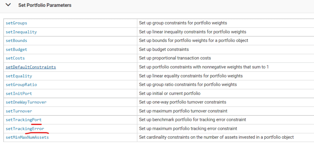
Even a simple example is illustrated about how to set up a portfolio, and parameter setting on cov, mean, ..to tracking error calculation. The codes beneath it is not revealed. Regard this inquiry, this article is far more satisfying: Trade Optimization by Corey Hoffstein on 2018.
#Trade optimization
import numpy
import pandas
from pulp import *
import scipy.optimize
# setup some sample data
tickers = "amj bkln bwx cwb emlc hyg idv lqd \
           pbp pcy pff rem shy tlt vnq vnqi vym".split()
w_target = pandas.Series([float(x) for x in "0.04095391 0.206519656 0 \
                      0.061190655 0.049414401 0.105442705 0.038080766 \
                      0.07004622 0.045115708 0.08508047 0.115974239 \
                      0.076953702 0 0.005797291 0.008955226 0.050530852 \
                      0.0399442".split()], index = tickers)
w_old = pandas.Series([float(x) for x in \
                   "0.058788745 0.25 0 0.098132817 \
                    0 0.134293993 0.06144967 0.102295438 \
                    0.074200473 0 0 0.118318536 0 0 \
                    0.04774768 0 0.054772649".split()], \
                      index = tickers)
n = len(tickers)
w_diff = w_target - w_old

# Try a naive optimization with SLSQP
theta = 0.05
theta_hat = theta + w_diff.abs().sum() / 2.
def _fmin(t):
    return numpy.sum(numpy.abs(t) > 1e-8)
def _distance_constraint(t):
    return theta_hat - numpy.sum(numpy.abs(t)) / 2.
def _sums_to_zero(t):
    return numpy.sum(numpy.square(t))
t0 = w_diff.copy()
bounds = [(-w_old[i], 1) for i in range(0, n)]
result = scipy.optimize.fmin_slsqp(_fmin, t0, bounds = bounds, \
                                   eqcons = [_sums_to_zero], \
                                   ieqcons = [_distance_constraint], \
                                   disp = -1)
result =  pandas.Series(result, index = tickers)

# Now try PuLP
lp_problem = LpProblem("Absolute Values", LpMinimize)
x_vars = []
psi_vars = []
bounds = [[1, 7], [-10, 0], [-9, -1], [-1, 5], [6, 9]]
print("Bounds for x: ")
print(pandas.DataFrame(bounds, columns = ["Left", "Right"]))
for i in range(5):
    x_i = LpVariable("x_" + str(i), None, None)
    x_vars.append(x_i)

    psi_i = LpVariable("psi_i" + str(i), None, None)
    psi_vars.append(psi_i)

lp_problem += lpSum(psi_vars), "Objective"
for i in range(5):
    lp_problem += psi_vars[i] >= -x_vars[i]
    lp_problem += psi_vars[i] >= x_vars[i]

    lp_problem += x_vars[i] >= bounds[i][0]
    lp_problem += x_vars[i] <= bounds[i][1]

lp_problem.solve()
print "\nx variables"
print pandas.Series([x_i.value() for x_i in x_vars])
print "\npsi Variables (|x|):"
print pandas.Series([psi_i.value() for psi_i in psi_vars])
Next, to build a minimization trade model, then sector rotation model. Powerful it is, linear programing has its limitation, the major one is quadratic constraints or objectives, such as tracking error constraints, are forbidden.
#non-linear optimization

covariance_matrix = [[ 3.62767735e-02,  2.18757921e-03,  2.88389154e-05,
         7.34489308e-03,  1.96701876e-03,  4.42465667e-03,
         1.12579361e-02,  1.65860525e-03,  5.64030644e-03,
         2.76645571e-03,  3.63015800e-04,  3.74241173e-03,
        -1.35199744e-04, -2.19000672e-03,  6.80914121e-03,
         8.41701096e-03,  1.07504229e-02],
       [ 2.18757921e-03,  5.40346050e-04,  5.52196510e-04,
         9.03853792e-04,  1.26047511e-03,  6.54178355e-04,
         1.72005989e-03,  3.60920296e-04,  4.32241813e-04,
         6.55664695e-04,  1.60990263e-04,  6.64729334e-04,
        -1.34505970e-05, -3.61651337e-04,  6.56663689e-04,
         1.55184724e-03,  1.06451898e-03],
       [ 2.88389154e-05,  5.52196510e-04,  4.73857357e-03,
         1.55701811e-03,  6.22138578e-03,  8.13498400e-04,
         3.36654245e-03,  1.54941008e-03,  6.19861236e-05,
         2.93028853e-03,  8.70115005e-04,  4.90113403e-04,
         1.22200026e-04,  2.34074752e-03,  1.39606650e-03,
         5.31970717e-03,  8.86435533e-04],
       [ 7.34489308e-03,  9.03853792e-04,  1.55701811e-03,
         4.70643696e-03,  2.36059044e-03,  1.45119740e-03,
         4.46141908e-03,  8.06488179e-04,  2.09341490e-03,
         1.54107719e-03,  6.99000273e-04,  1.31596059e-03,
        -2.52039718e-05, -5.18390335e-04,  2.41334278e-03,
         5.14806453e-03,  3.76769305e-03],
       [ 1.96701876e-03,  1.26047511e-03,  6.22138578e-03,
         2.36059044e-03,  1.26644146e-02,  2.00358907e-03,
         8.04023724e-03,  2.30076077e-03,  5.70077091e-04,
         5.65049374e-03,  9.76571021e-04,  1.85279450e-03,
         2.56652171e-05,  1.19266940e-03,  5.84713900e-04,
         9.29778319e-03,  2.84300900e-03],
       [ 4.42465667e-03,  6.54178355e-04,  8.13498400e-04,
         1.45119740e-03,  2.00358907e-03,  1.52522064e-03,
         2.91651452e-03,  8.70569737e-04,  1.09752760e-03,
         1.66762294e-03,  5.36854007e-04,  1.75343988e-03,
         1.29714019e-05,  9.11071171e-05,  1.68043070e-03,
         2.42628131e-03,  1.90713194e-03],
       [ 1.12579361e-02,  1.72005989e-03,  3.36654245e-03,
         4.46141908e-03,  8.04023724e-03,  2.91651452e-03,
         1.19931947e-02,  1.61222907e-03,  2.75699780e-03,
         4.16113427e-03,  6.25609018e-04,  2.91008175e-03,
        -1.92908806e-04, -1.57151126e-03,  3.25855486e-03,
         1.06990068e-02,  6.05007409e-03],
       [ 1.65860525e-03,  3.60920296e-04,  1.54941008e-03,
         8.06488179e-04,  2.30076077e-03,  8.70569737e-04,
         1.61222907e-03,  1.90797844e-03,  6.04486114e-04,
         2.47501106e-03,  8.57227194e-04,  2.42587888e-03,
         1.85623409e-04,  2.91479004e-03,  3.33754926e-03,
         2.61280946e-03,  1.16461350e-03],
       [ 5.64030644e-03,  4.32241813e-04,  6.19861236e-05,
         2.09341490e-03,  5.70077091e-04,  1.09752760e-03,
         2.75699780e-03,  6.04486114e-04,  2.53455649e-03,
         9.66091919e-04,  3.91053383e-04,  1.83120456e-03,
        -4.91230334e-05, -5.60316891e-04,  2.28627416e-03,
         2.40776877e-03,  3.15907037e-03],
       [ 2.76645571e-03,  6.55664695e-04,  2.93028853e-03,
         1.54107719e-03,  5.65049374e-03,  1.66762294e-03,
         4.16113427e-03,  2.47501106e-03,  9.66091919e-04,
         4.81734656e-03,  1.14396535e-03,  3.23711266e-03,
         1.69157413e-04,  3.03445975e-03,  3.09323955e-03,
         5.27456576e-03,  2.11317800e-03],
       [ 3.63015800e-04,  1.60990263e-04,  8.70115005e-04,
         6.99000273e-04,  9.76571021e-04,  5.36854007e-04,
         6.25609018e-04,  8.57227194e-04,  3.91053383e-04,
         1.14396535e-03,  1.39905835e-03,  2.01826986e-03,
         1.04811491e-04,  1.67653296e-03,  2.59598793e-03,
         1.01532651e-03,  2.60716967e-04],
       [ 3.74241173e-03,  6.64729334e-04,  4.90113403e-04,
         1.31596059e-03,  1.85279450e-03,  1.75343988e-03,
         2.91008175e-03,  2.42587888e-03,  1.83120456e-03,
         3.23711266e-03,  2.01826986e-03,  1.16861730e-02,
         2.24795908e-04,  3.46679680e-03,  8.38606091e-03,
         3.65575720e-03,  1.80220367e-03],
       [-1.35199744e-04, -1.34505970e-05,  1.22200026e-04,
        -2.52039718e-05,  2.56652171e-05,  1.29714019e-05,
        -1.92908806e-04,  1.85623409e-04, -4.91230334e-05,
         1.69157413e-04,  1.04811491e-04,  2.24795908e-04,
         5.49990619e-05,  5.01897963e-04,  3.74856789e-04,
        -8.63113243e-06, -1.51400879e-04],
       [-2.19000672e-03, -3.61651337e-04,  2.34074752e-03,
        -5.18390335e-04,  1.19266940e-03,  9.11071171e-05,
        -1.57151126e-03,  2.91479004e-03, -5.60316891e-04,
         3.03445975e-03,  1.67653296e-03,  3.46679680e-03,
         5.01897963e-04,  8.74709395e-03,  6.37760454e-03,
         1.74349274e-03, -1.26348683e-03],
       [ 6.80914121e-03,  6.56663689e-04,  1.39606650e-03,
         2.41334278e-03,  5.84713900e-04,  1.68043070e-03,
         3.25855486e-03,  3.33754926e-03,  2.28627416e-03,
         3.09323955e-03,  2.59598793e-03,  8.38606091e-03,
         3.74856789e-04,  6.37760454e-03,  1.55034038e-02,
         5.20888498e-03,  4.17926704e-03],
       [ 8.41701096e-03,  1.55184724e-03,  5.31970717e-03,
         5.14806453e-03,  9.29778319e-03,  2.42628131e-03,
         1.06990068e-02,  2.61280946e-03,  2.40776877e-03,
         5.27456576e-03,  1.01532651e-03,  3.65575720e-03,
        -8.63113243e-06,  1.74349274e-03,  5.20888498e-03,
         1.35424275e-02,  5.49882762e-03],
       [ 1.07504229e-02,  1.06451898e-03,  8.86435533e-04,
         3.76769305e-03,  2.84300900e-03,  1.90713194e-03,
         6.05007409e-03,  1.16461350e-03,  3.15907037e-03,
         2.11317800e-03,  2.60716967e-04,  1.80220367e-03,
        -1.51400879e-04, -1.26348683e-03,  4.17926704e-03,
         5.49882762e-03,  7.08734925e-03]]
covariance_matrix = pandas.DataFrame(covariance_matrix, \
                                     index = tickers, \
                                     columns = tickers)
theta = 0.05
target_te = 0.0025
w_old_prime = w_old.copy()
# calculate the difference from the target portfolio
# and use this difference to estimate tracking error
# and marginal contribution to tracking error ("mcte")
z = (w_old_prime - w_target)
te = numpy.sqrt(z.dot(covariance_matrix).dot(z))
mcte = (z.dot(covariance_matrix)) / te
while True:
    w_diff_prime = w_target - w_old_prime
    trading_model = LpProblem("Trade Minimization Problem", LpMinimize)
    t_vars = []
    psi_vars = []
    phi_vars = []
    y_vars = []
    A = 2
    for i in range(n):
        t = LpVariable("t_" + str(i), -w_old_prime[i], 1 - w_old_prime[i])
        t_vars.append(t)
        psi = LpVariable("psi_" + str(i), None, None)
        psi_vars.append(psi)
        phi = LpVariable("phi_" + str(i), None, None)
        phi_vars.append(phi)
        y = LpVariable("y_" + str(i), 0, 1, LpInteger) #set y in {0, 1}
        y_vars.append(y)
    # add our objective to minimize y, which is the number of trades
    trading_model += lpSum(phi_vars) + lpSum(y_vars), "Objective"
    for i in range(n):
        trading_model += psi_vars[i] >= -t_vars[i]
        trading_model += psi_vars[i] >= t_vars[i]
        trading_model += psi_vars[i] <= A * y_vars[i]
    for i in range(n):
        trading_model += phi_vars[i] >= -(w_diff_prime[i] - t_vars[i])
        trading_model += phi_vars[i] >= (w_diff_prime[i] - t_vars[i])
    # Make sure our trades sum to zero
    trading_model += (lpSum(t_vars) == 0)

    # Set tracking error limit
    #    delta(te) = mcte * delta(z)
    #              = mcte * ((w_old_prime + t - w_target) -
    #                        (w_old_prime - w_target))
    #              = mcte * t
    #    te + delta(te) <= target_te
    #    ==> delta(te) <= target_te - te
    trading_model += (lpSum([mcte.iloc[i] * t_vars[i] for i in range(n)]) \
                              <= (target_te - te))
    # Set our trade bounds
    trading_model += (lpSum(phi_vars) / 2. <= theta)
    trading_model.solve()

    # update our w_old' with the current trades
    results = pandas.Series([t_i.value() for t_i in t_vars], index = tickers)
    w_old_prime = (w_old_prime + results)

    z = (w_old_prime - w_target)
    te = numpy.sqrt(z.dot(covariance_matrix).dot(z))
    mcte = (z.dot(covariance_matrix)) / te

    if te < target_te:
        break

print "Tracking error: " + str(te)
# since w_old' is an iterative update,
# the current trades only reflect the updates from
# the prior w_old'.  Thus, we need to calculate
# the trades by hand
results = (w_old_prime - w_old)
n_trades = (results.abs() > 1e-8).astype(int).sum()
print "Number of trades: " + str(n_trades)
print "Turnover distance: " + str((w_target - (w_old + results)).abs().sum() / 2.)
The author discussed in last paragraph that Constraints within the practice of trade optimization typically fall into one of three categories: asset paring, trade paring, and level paring. “
Asset paring restricts the number of securities the portfolio can hold, trade paring restricts the number of trades that can be made, and level paring restricts the size of positions and trades. Introducing these constraints often turns an optimization into a discrete problem, making it much more difficult to solve for traditional convex optimizations.
With this in mind, we introduced mixed-integer linear programming (“MILP”) and explore a few techniques that can be utilized to transform non-linear functions into a set of linear constraints. We then combined these transformations to develop a simple trade optimization framework that can be solved using MILP optimizers.
To offer numerical support in the discussion, we created a simple momentum-based sector rotation strategy. We found that naive turnover-filtering helped reduce the number of trades executed by 50%, while explicit trade optimization reduced the number of trades by 70%.
Finally, we explored how our simplified framework could be further extended to account for both non-linear functional constraints (e.g. tracking error) and operational constraints (e.g. managing execution time).
The paring constraints introduced by trade optimization often lead to problems that are difficult to solve. However, when we consider that the cost of trading is a very real drag on the results realized by investors, we believe that the solutions are worth pursuing.”
