For example,

This is intuitive however we need to apply the chain rule as is taught, and expandable to be used in more complex scenarios. On this topic, Prof.Shifrin provided a thorough explanation:

Use this as an example, suppose f is a differentiable function on the plane and it satisfies

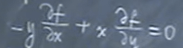
This is actually same as the below function, but how can we discover this?

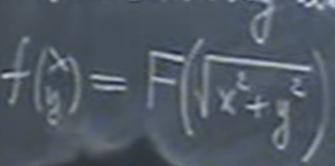
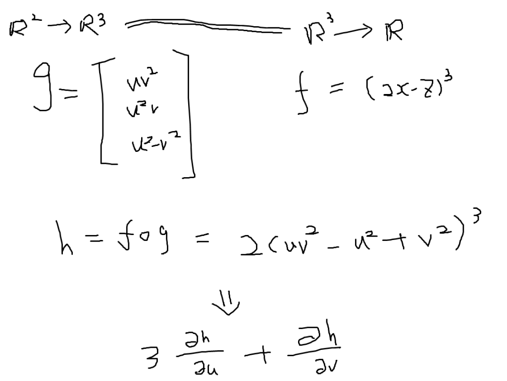
Here is the answer: consider big F as fog:

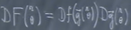
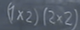
After the calculation, we reach

Two more problems to try out the concept understanding.

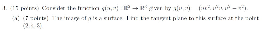
Q1. Find the tangent plane (give me the equation) for the below surface at the specified point

Q2. What is the surface function f to describe the below relationship between x, y and z? Given a point (a, b, c) on this surface find the tangent plane equation.

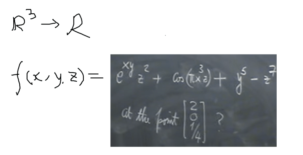
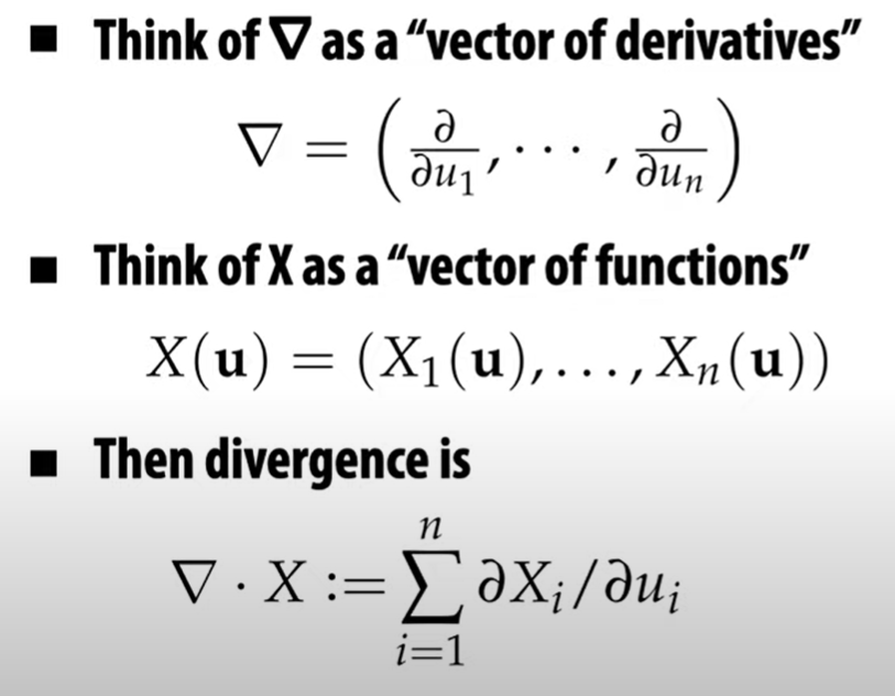
Question, does gradient always to define R^n to R? the answer is yes. according to wiki, “the gradient of a scalar-valued differentiable function f of several variables is the vector field (or vector-valued function) f whose value at a point p is the vector[a] whose components are the partial derivatives of p. It’s so gibberish from wiki, to have a deep understanding, I add on course from Keenan Crane, and deduce the following from basic concepts of derivative and gradient:

Once grasped this concept, let’s try to think what is the gradient of a function of a function – L² Gradient?

For example,

going through the basic concept, it’s not hard to deduce above.

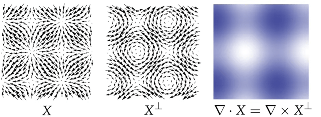
Divergence’s understanding also can be taken in a fresh new perspective: in stead of thinking it as flux measurement, think of it as furthering “gradient of scalar function phi” to “gradient of gradient(vector field)”.

From R2 –> R2, Polar system to Cartesian system, f(x, y) = f(rcos(theta), rsin(theta)) if we say there is such a relationship x squared + y squared then this function is to be directed from R2 to R(scaler), and it can be more conveniently expressed as or (rcos(theta))^2 + (rsin(theta))^2 = r^2. So this problem is essentially R2 –> R2 –> R problem.

Adding on another similar questions from HW#6 no.3

it’s an R2 but asked as a R3.

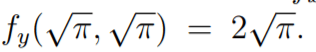
fx = fy easy to compute, cut screenshot below, fz = -1 as it can be written as F(x, y, z)

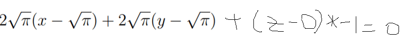
Given any point on the tangent plane (x, y, z), minus the point given (square root pie, square root pie, 0),

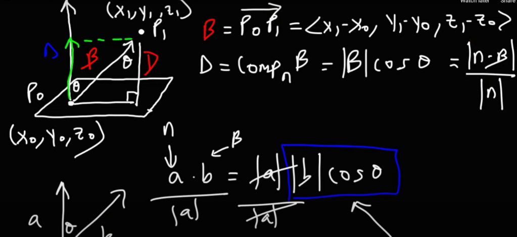
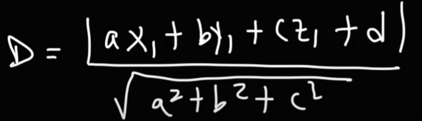
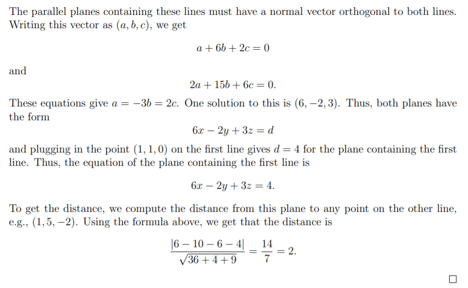
Add on Nov30 2021 fundamental concepts on finding the distance from the point to a plane: It is actually a bit tricky – requiring some math cleverness to deduce

That’s why for HW#2, problem 2,

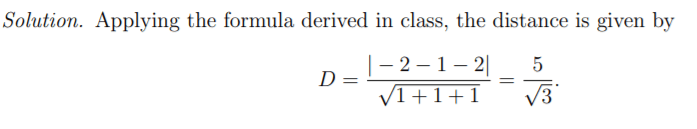
To find whether the point is above or below the plane, we can look for a point in the plane
with the same x and y values. Plugging those in, we want −2 − 1 + z = 2 so that z = 5. Since
this is larger than the z coordinate of the point, the point is below the plane.

Next try to solve the distance between two lines or two planes. First you need to judge if the two lines are parallel, or intersected. Then convert the problem to point to plane problem as above.

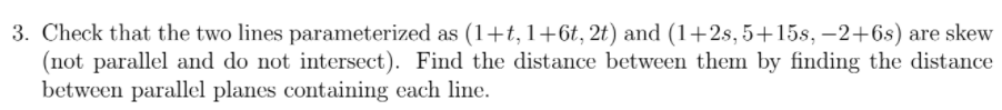
Vectors parallel to the two lines are (1, 6, 2) and (2, 15, 6), respectively, so the lines are not parallel since these are not scalar multiples.

If we had an intersection point, we would have
1 + t = 1 + 2s
1 + 6t = 5 + 15s
and
2t = −2 + 6s.
Solving the first and third equations gives t = 2, s = 1 which does not satisfy the second
equation. Thus, we have shown that these lines are skew.

Then we need to find distance,

Adding on a HW problem to further understand the concept of R2 contour map:

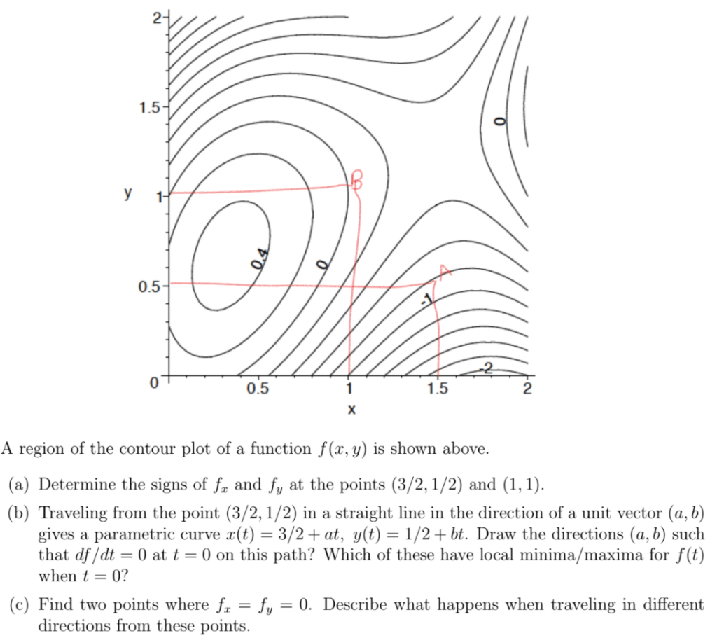
(symbol in math is of vital importance, know what it means, fx means the partial derivative on x)

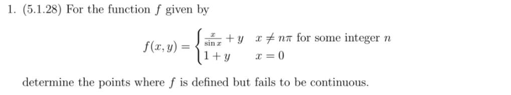
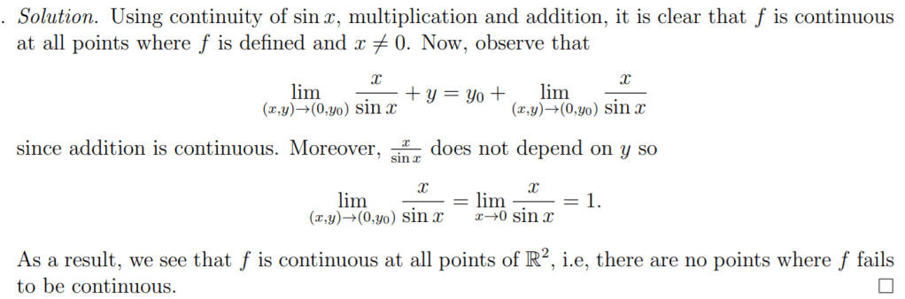
From HW#6 to deepen the concept of “continuous” in calculus. In mathematics, a continuous function is a function that does not have any abrupt changes in value, known as discontinuities. More precisely, a function is continuous if arbitrarily small changes in its output can be assured by restricting to sufficiently small changes in its input.

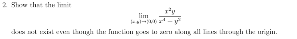
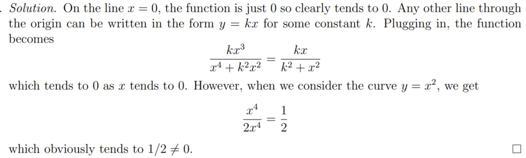
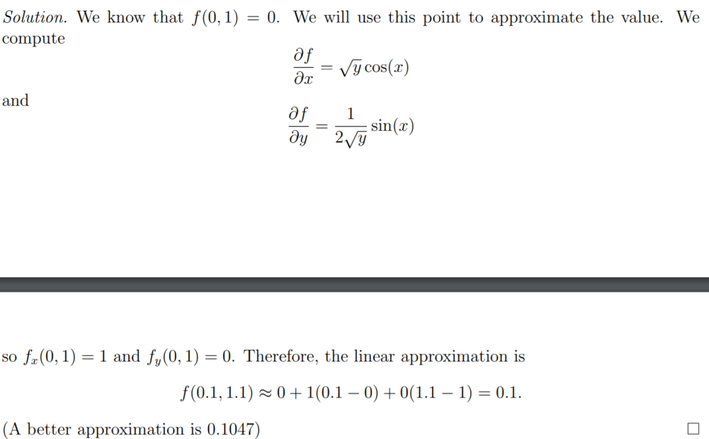
Approximation is also an essence of calculus together with limit and continuity. For example

It’s hard to compute directly so let’s compute f(0, 1)=0 and then approximate

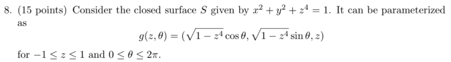
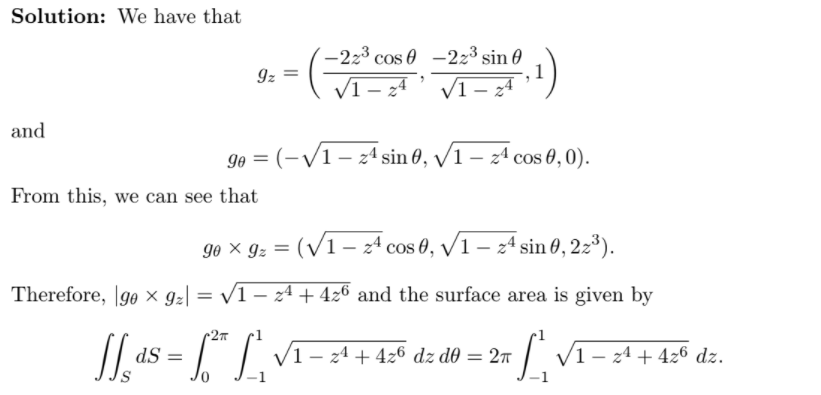
Another example of very close observation and understanding is the variable form in surface integral. In one problem, canonical form is z, theta two parameters mapped to x, y, z three parameters:

You can just plug in formula as taught in textbook.

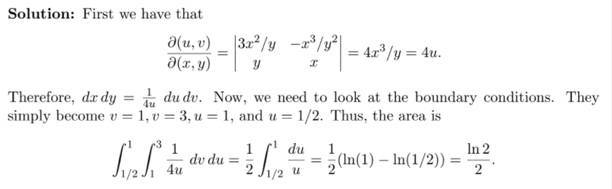
With a little bit variation, such as this problem:

Note the u, v mapping to x, y is not expressed in u, v but in x and y here. If you want to follow the above example, it’s very difficult to calculate the g_u and g_v, however, the form in x, y is easy, i.e., it’s easy to compute the fx and fy, but then you need to reverse it!

Above solution is given by the teacher, but I think the following would be more lucid: