Scipy has an optimize package that greatly supplement PuLP I tried to conquer the problem of optimizing portfolio, and more concretely to my current workflow – to optimize the weights of a given portfolio.
So the first step is to have a high-level good understanding of Scipy package’s Optimize functions. One can always type “help(scipy.optimize)” for help in command environment.
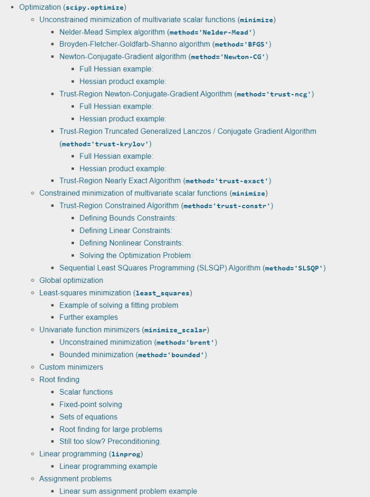
The key focus is Sequential Least SQuares Programming (SLSQP) Algorithm (method=’SLSQP’). It aims to solve kind of problems as such:
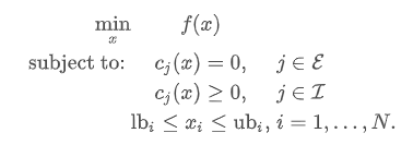
An example provided by the official source is as follows:
from scipy.optimize import minimize
def rosen(x):
    """The Rosenbrock function"""
    return sum(100.0*(x[1:]-x[:-1]**2.0)**2.0 + (1-x[:-1])**2.0)
# the Rosenbrock function is a non-convex function, introduced by Howard H. Rosenbrock in 1960, which is used as a performance test problem for optimization algorithms.[1] It is also known as Rosenbrock's valley or Rosenbrock's banana function.
# f(x,y)=(a-x)^{2}+b(y-x^{2})^{2}
def rosen_der(x):
    xm = x[1:-1]
    xm_m1 = x[:-2]
    xm_p1 = x[2:]
    der = np.zeros_like(x)
    der[1:-1] = 200*(xm-xm_m1**2) - 400*(xm_p1 - xm**2)*xm - 2*(1-xm)
    der[0] = -400*x[0]*(x[1]-x[0]**2) - 2*(1-x[0])
    der[-1] = 200*(x[-1]-x[-2]**2)
    return der

ineq_cons = {'type': 'ineq',
             'fun' : lambda x: np.array([1 - x[0] - 2*x[1],
                                         1 - x[0]**2 - x[1],
                                         1 - x[0]**2 + x[1]]),
             'jac' : lambda x: np.array([[-1.0, -2.0],
                                         [-2*x[0], -1.0],
                                         [-2*x[0], 1.0]])}
eq_cons = {'type': 'eq',
           'fun' : lambda x: np.array([2*x[0] + x[1] - 1]),
           'jac' : lambda x: np.array([2.0, 1.0])}
from scipy.optimize import Bounds
bounds = Bounds([0, -0.5], [1.0, 2.0])
x0 = np.array([0.5, 0])
res = minimize(rosen, x0, method='SLSQP', jac=rosen_der,
               constraints=[eq_cons, ineq_cons], options={'ftol': 1e-9, 'disp': True},
               bounds=bounds)
# Optimization terminated successfully    (Exit mode 0)
#             Current function value: 0.34271757499419825
#             Iterations: 4
#             Function evaluations: 5
#             Gradient evaluations: 4
# from Vijay, who already put the weights optimization functions using scipy, I can reference direclty:
from scipy.optimize import minimize
def portfolio_vol(weights, covmat):
    """
    Computes the vol of a portfolio from a covariance matrix and constituent weights
    weights are a numpy array or N x 1 maxtrix and covmat is an N x N matrix
    """
    return (weights.T @ covmat @ weights)**0.5

def minimize_vol(target_return, er, cov):
    """
    Returns the optimal weights that achieve the target return
    given a set of expected returns and a covariance matrix
    """
    n = er.shape[0]
    init_guess = np.repeat(1/n, n)
    bounds = ((0.0, 1.0),) * n # an N-tuple of 2-tuples!
    # construct the constraints
    weights_sum_to_1 = {'type': 'eq',
                        'fun': lambda weights: np.sum(weights) - 1
    }
    return_is_target = {'type': 'eq',
                        'args': (er,),
                        'fun': lambda weights, er: target_return - portfolio_return(weights,er)
    }
    weights = minimize(portfolio_vol, init_guess,
                       args=(cov,), method='SLSQP',
                       options={'disp': False},
                       constraints=(weights_sum_to_1,return_is_target),
                       bounds=bounds)
    return weights.x
