The essence of portfolio management is set stone by Markowitz by his brilliance two-assets frontier plot, stating and approving an optimized portfolio can be achieve simply by adjusting the weights lowering the volatility/risk and increasing the expected return.
In Vijay’s data, he used a history from 1996 to 2003 of 30 industries.

cov = ind30['1996': '2000'].cov()
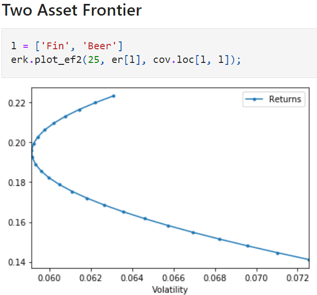
So set an expected return on the graph above, then we can run optimization algo to find the best combination of weights achieving lowest volatility. This is the min-vol strategy!
Here are the full codes from Vijay github for full reference purpose. With regard to this min-vol strategy, the key components are portfolio_return, portfolio_vol, minimize_vol, andmsr (Returns the weights of the portfolio that gives you the maximum sharpe ratio given the riskfree rate and expected returns and a covariance matrix).
It’s worth noting that the objective in minimize_vol function itself is a function “portfolio_vol”, which takes two argument, weights and covmat, weights is exact in constraints, while the other argument covmat is set to be “args = (cov,_) in the minimize parameters.


import pandas as pd
import numpy as np
import math
from scipy.stats import norm

def get_ffme_returns():
    """
    Load the Fama-French Dataset for the returns of the Top and Bottom Deciles by MarketCap
    """
    me_m = pd.read_csv("data/Portfolios_Formed_on_ME_monthly_EW.csv",
                       header=0, index_col=0, na_values=-99.99)
    rets = me_m[['Lo 10', 'Hi 10']]
    rets.columns = ['SmallCap', 'LargeCap']
    rets = rets/100
    rets.index = pd.to_datetime(rets.index, format="%Y%m").to_period('M')
    return rets


def get_hfi_returns():
    """
    Load and format the EDHEC Hedge Fund Index Returns
    """
    hfi = pd.read_csv("data/edhec-hedgefundindices.csv",
                      header=0, index_col=0, parse_dates=True)
    hfi = hfi/100
    hfi.index = hfi.index.to_period('M')
    return hfi

def get_ind_file(filetype):
    """
    Load and format the Ken French 30 Industry Portfolios files
    """
    known_types = ["returns", "nfirms", "size"]
    if filetype not in known_types:
        sep = ','
        raise ValueError(f'filetype must be one of:{sep.join(known_types)}')
    if filetype is "returns":
        name = "vw_rets"
        divisor = 100
    elif filetype is "nfirms":
        name = "nfirms"
        divisor = 1
    elif filetype is "size":
        name = "size"
        divisor = 1
    ind = pd.read_csv(f"data/ind30_m_{name}.csv", header=0, index_col=0)/divisor
    ind.index = pd.to_datetime(ind.index, format="%Y%m").to_period('M')
    ind.columns = ind.columns.str.strip()
    return ind

def get_ind_returns():
    """
    Load and format the Ken French 30 Industry Portfolios Value Weighted Monthly Returns
    """
    return get_ind_file("returns")

def get_ind_nfirms():
    """
    Load and format the Ken French 30 Industry Portfolios Average number of Firms
    """
    return get_ind_file("nfirms")

def get_ind_size():
    """
    Load and format the Ken French 30 Industry Portfolios Average size (market cap)
    """
    return get_ind_file("size")


def get_total_market_index_returns():
    """
    Load the 30 industry portfolio data and derive the returns of a capweighted total market index
    """
    ind_nfirms = get_ind_nfirms()
    ind_size = get_ind_size()
    ind_return = get_ind_returns()
    ind_mktcap = ind_nfirms * ind_size
    total_mktcap = ind_mktcap.sum(axis=1)
    ind_capweight = ind_mktcap.divide(total_mktcap, axis="rows")
    total_market_return = (ind_capweight * ind_return).sum(axis="columns")
    return total_market_return

def skewness(r):
    """
    Alternative to scipy.stats.skew()
    Computes the skewness of the supplied Series or DataFrame
    Returns a float or a Series
    """
    demeaned_r = r - r.mean()
    # use the population standard deviation, so set dof=0
    sigma_r = r.std(ddof=0)
    exp = (demeaned_r**3).mean()
    return exp/sigma_r**3


def kurtosis(r):
    """
    Alternative to scipy.stats.kurtosis()
    Computes the kurtosis of the supplied Series or DataFrame
    Returns a float or a Series
    """
    demeaned_r = r - r.mean()
    # use the population standard deviation, so set dof=0
    sigma_r = r.std(ddof=0)
    exp = (demeaned_r**4).mean()
    return exp/sigma_r**4


def compound(r):
    """
    returns the result of compounding the set of returns in r
    """
    return np.expm1(np.log1p(r).sum())


def annualize_rets(r, periods_per_year):
    """
    Annualizes a set of returns
    We should infer the periods per year
    but that is currently left as an exercise
    to the reader 🙂
    """
    compounded_growth = (1+r).prod()
    n_periods = r.shape[0]
    return compounded_growth**(periods_per_year/n_periods)-1


def annualize_vol(r, periods_per_year):
    """
    Annualizes the vol of a set of returns
    We should infer the periods per year
    but that is currently left as an exercise
    to the reader 🙂
    """
    return r.std()*(periods_per_year**0.5)


def sharpe_ratio(r, riskfree_rate, periods_per_year):
    """
    Computes the annualized sharpe ratio of a set of returns
    """
    # convert the annual riskfree rate to per period
    rf_per_period = (1+riskfree_rate)**(1/periods_per_year)-1
    excess_ret = r - rf_per_period
    ann_ex_ret = annualize_rets(excess_ret, periods_per_year)
    ann_vol = annualize_vol(r, periods_per_year)
    return ann_ex_ret/ann_vol


import scipy.stats
def is_normal(r, level=0.01):
    """
    Applies the Jarque-Bera test to determine if a Series is normal or not
    Test is applied at the 1% level by default
    Returns True if the hypothesis of normality is accepted, False otherwise
    """
    if isinstance(r, pd.DataFrame):
        return r.aggregate(is_normal)
    else:
        statistic, p_value = scipy.stats.jarque_bera(r)
        return p_value > level


def drawdown(return_series: pd.Series):
    """Takes a time series of asset returns.
       returns a DataFrame with columns for
       the wealth index,
       the previous peaks, and
       the percentage drawdown
    """
    wealth_index = 1000*(1+return_series).cumprod()
    previous_peaks = wealth_index.cummax()
    drawdowns = (wealth_index - previous_peaks)/previous_peaks
    return pd.DataFrame({"Wealth": wealth_index,
                         "Previous Peak": previous_peaks,
                         "Drawdown": drawdowns})


def semideviation(r):
    """
    Returns the semideviation aka negative semideviation of r
    r must be a Series or a DataFrame, else raises a TypeError
    """
    if isinstance(r, pd.Series):
        is_negative = r < 0
        return r[is_negative].std(ddof=0)
    elif isinstance(r, pd.DataFrame):
        return r.aggregate(semideviation)
    else:
        raise TypeError("Expected r to be a Series or DataFrame")


def var_historic(r, level=5):
    """
    Returns the historic Value at Risk at a specified level
    i.e. returns the number such that "level" percent of the returns
    fall below that number, and the (100-level) percent are above
    """
    if isinstance(r, pd.DataFrame):
        return r.aggregate(var_historic, level=level)
    elif isinstance(r, pd.Series):
        return -np.percentile(r, level)
    else:
        raise TypeError("Expected r to be a Series or DataFrame")


def cvar_historic(r, level=5):
    """
    Computes the Conditional VaR of Series or DataFrame
    """
    if isinstance(r, pd.Series):
        is_beyond = r <= -var_historic(r, level=level)
        return -r[is_beyond].mean()
    elif isinstance(r, pd.DataFrame):
        return r.aggregate(cvar_historic, level=level)
    else:
        raise TypeError("Expected r to be a Series or DataFrame")

def var_gaussian(r, level=5, modified=False):
    """
    Returns the Parametric Gauusian VaR of a Series or DataFrame
    If "modified" is True, then the modified VaR is returned,
    using the Cornish-Fisher modification
    """
    # compute the Z score assuming it was Gaussian
    z = norm.ppf(level/100)
    if modified:
        # modify the Z score based on observed skewness and kurtosis
        s = skewness(r)
        k = kurtosis(r)
        z = (z +
                (z**2 - 1)*s/6 +
                (z**3 -3*z)*(k-3)/24 -
                (2*z**3 - 5*z)*(s**2)/36
            )
    return -(r.mean() + z*r.std(ddof=0))


def portfolio_return(weights, returns):
    """
    Computes the return on a portfolio from constituent returns and weights
    weights are a numpy array or Nx1 matrix and returns are a numpy array or Nx1 matrix
    """
    return weights.T @ returns


def portfolio_vol(weights, covmat):
    """
    Computes the vol of a portfolio from a covariance matrix and constituent weights
    weights are a numpy array or N x 1 maxtrix and covmat is an N x N matrix
    """
    return (weights.T @ covmat @ weights)**0.5


def plot_ef2(n_points, er, cov):
    """
    Plots the 2-asset efficient frontier
    """
    if er.shape[0] != 2 or er.shape[0] != 2:
        raise ValueError("plot_ef2 can only plot 2-asset frontiers")
    weights = [np.array([w, 1-w]) for w in np.linspace(0, 1, n_points)]
    rets = [portfolio_return(w, er) for w in weights]
    vols = [portfolio_vol(w, cov) for w in weights]
    ef = pd.DataFrame({
        "Returns": rets,
        "Volatility": vols
    })
    return ef.plot.line(x="Volatility", y="Returns", style=".-")


from scipy.optimize import minimize

def minimize_vol(target_return, er, cov):
    """
    Returns the optimal weights that achieve the target return
    given a set of expected returns and a covariance matrix
    """
    n = er.shape[0]
    init_guess = np.repeat(1/n, n)
    bounds = ((0.0, 1.0),) * n # an N-tuple of 2-tuples!
    # construct the constraints
    weights_sum_to_1 = {'type': 'eq',
                        'fun': lambda weights: np.sum(weights) - 1
    }
    return_is_target = {'type': 'eq',
                        'args': (er,),
                        'fun': lambda weights, er: target_return - portfolio_return(weights,er)
    }
    weights = minimize(portfolio_vol, init_guess,
                       args=(cov,), method='SLSQP',
                       options={'disp': False},
                       constraints=(weights_sum_to_1,return_is_target),
                       bounds=bounds)
    return weights.x


def msr(riskfree_rate, er, cov):
    """
    Returns the weights of the portfolio that gives you the maximum sharpe ratio
    given the riskfree rate and expected returns and a covariance matrix
    """
    n = er.shape[0]
    init_guess = np.repeat(1/n, n)
    bounds = ((0.0, 1.0),) * n # an N-tuple of 2-tuples!
    # construct the constraints
    weights_sum_to_1 = {'type': 'eq',
                        'fun': lambda weights: np.sum(weights) - 1
    }
    def neg_sharpe(weights, riskfree_rate, er, cov):
        """
        Returns the negative of the sharpe ratio
        of the given portfolio
        """
        r = portfolio_return(weights, er)
        vol = portfolio_vol(weights, cov)
        return -(r - riskfree_rate)/vol

    weights = minimize(neg_sharpe, init_guess,
                       args=(riskfree_rate, er, cov), method='SLSQP',
                       options={'disp': False},
                       constraints=(weights_sum_to_1,),
                       bounds=bounds)
    return weights.x


def gmv(cov):
    """
    Returns the weights of the Global Minimum Volatility portfolio
    given a covariance matrix
    """
    n = cov.shape[0]
    return msr(0, np.repeat(1, n), cov)


def optimal_weights(n_points, er, cov):
    """
    Returns a list of weights that represent a grid of n_points on the efficient frontier
    """
    target_rs = np.linspace(er.min(), er.max(), n_points)
    weights = [minimize_vol(target_return, er, cov) for target_return in target_rs]
    return weights


def plot_ef(n_points, er, cov, style='.-', legend=False, show_cml=False, riskfree_rate=0, show_ew=False, show_gmv=False):
    """
    Plots the multi-asset efficient frontier
    """
    weights = optimal_weights(n_points, er, cov)
    rets = [portfolio_return(w, er) for w in weights]
    vols = [portfolio_vol(w, cov) for w in weights]
    ef = pd.DataFrame({
        "Returns": rets,
        "Volatility": vols
    })
    ax = ef.plot.line(x="Volatility", y="Returns", style=style, legend=legend)
    if show_cml:
        ax.set_xlim(left = 0)
        # get MSR
        w_msr = msr(riskfree_rate, er, cov)
        r_msr = portfolio_return(w_msr, er)
        vol_msr = portfolio_vol(w_msr, cov)
        # add CML
        cml_x = [0, vol_msr]
        cml_y = [riskfree_rate, r_msr]
        ax.plot(cml_x, cml_y, color='green', marker='o', linestyle='dashed', linewidth=2, markersize=10)
    if show_ew:
        n = er.shape[0]
        w_ew = np.repeat(1/n, n)
        r_ew = portfolio_return(w_ew, er)
        vol_ew = portfolio_vol(w_ew, cov)
        # add EW
        ax.plot([vol_ew], [r_ew], color='goldenrod', marker='o', markersize=10)
    if show_gmv:
        w_gmv = gmv(cov)
        r_gmv = portfolio_return(w_gmv, er)
        vol_gmv = portfolio_vol(w_gmv, cov)
        # add EW
        ax.plot([vol_gmv], [r_gmv], color='midnightblue', marker='o', markersize=10)

        return ax


def run_cppi(risky_r, safe_r=None, m=3, start=1000, floor=0.8, riskfree_rate=0.03, drawdown=None):
    """
    Run a backtest of the CPPI strategy, given a set of returns for the risky asset
    Returns a dictionary containing: Asset Value History, Risk Budget History, Risky Weight History
    """
    # set up the CPPI parameters
    dates = risky_r.index
    n_steps = len(dates)
    account_value = start
    floor_value = start*floor
    peak = account_value
    if isinstance(risky_r, pd.Series):
        risky_r = pd.DataFrame(risky_r, columns=["R"])

    if safe_r is None:
        safe_r = pd.DataFrame().reindex_like(risky_r)
        safe_r.values[:] = riskfree_rate/12 # fast way to set all values to a number
    # set up some DataFrames for saving intermediate values
    account_history = pd.DataFrame().reindex_like(risky_r)
    risky_w_history = pd.DataFrame().reindex_like(risky_r)
    cushion_history = pd.DataFrame().reindex_like(risky_r)
    floorval_history = pd.DataFrame().reindex_like(risky_r)
    peak_history = pd.DataFrame().reindex_like(risky_r)

    for step in range(n_steps):
        if drawdown is not None:
            peak = np.maximum(peak, account_value)
            floor_value = peak*(1-drawdown)
        cushion = (account_value - floor_value)/account_value
        risky_w = m*cushion
        risky_w = np.minimum(risky_w, 1)
        risky_w = np.maximum(risky_w, 0)
        safe_w = 1-risky_w
        risky_alloc = account_value*risky_w
        safe_alloc = account_value*safe_w
        # recompute the new account value at the end of this step
        account_value = risky_alloc*(1+risky_r.iloc[step]) + safe_alloc*(1+safe_r.iloc[step])
        # save the histories for analysis and plotting
        cushion_history.iloc[step] = cushion
        risky_w_history.iloc[step] = risky_w
        account_history.iloc[step] = account_value
        floorval_history.iloc[step] = floor_value
        peak_history.iloc[step] = peak
    risky_wealth = start*(1+risky_r).cumprod()
    backtest_result = {
        "Wealth": account_history,
        "Risky Wealth": risky_wealth,
        "Risk Budget": cushion_history,
        "Risky Allocation": risky_w_history,
        "m": m,
        "start": start,
        "floor": floor,
        "risky_r":risky_r,
        "safe_r": safe_r,
        "drawdown": drawdown,
        "peak": peak_history,
        "floor": floorval_history
    }
    return backtest_result


def summary_stats(r, riskfree_rate=0.03):
    """
    Return a DataFrame that contains aggregated summary stats for the returns in the columns of r
    """
    ann_r = r.aggregate(annualize_rets, periods_per_year=12)
    ann_vol = r.aggregate(annualize_vol, periods_per_year=12)
    ann_sr = r.aggregate(sharpe_ratio, riskfree_rate=riskfree_rate, periods_per_year=12)
    dd = r.aggregate(lambda r: drawdown(r).Drawdown.min())
    skew = r.aggregate(skewness)
    kurt = r.aggregate(kurtosis)
    cf_var5 = r.aggregate(var_gaussian, modified=True)
    hist_cvar5 = r.aggregate(cvar_historic)
    return pd.DataFrame({
        "Annualized Return": ann_r,
        "Annualized Vol": ann_vol,
        "Skewness": skew,
        "Kurtosis": kurt,
        "Cornish-Fisher VaR (5%)": cf_var5,
        "Historic CVaR (5%)": hist_cvar5,
        "Sharpe Ratio": ann_sr,
        "Max Drawdown": dd
    })


def gbm(n_years = 10, n_scenarios=1000, mu=0.07, sigma=0.15, steps_per_year=12, s_0=100.0, prices=True):
    """
    Evolution of Geometric Brownian Motion trajectories, such as for Stock Prices through Monte Carlo
    :param n_years:  The number of years to generate data for
    :param n_paths: The number of scenarios/trajectories
    :param mu: Annualized Drift, e.g. Market Return
    :param sigma: Annualized Volatility
    :param steps_per_year: granularity of the simulation
    :param s_0: initial value
    :return: a numpy array of n_paths columns and n_years*steps_per_year rows
    """
    # Derive per-step Model Parameters from User Specifications
    dt = 1/steps_per_year
    n_steps = int(n_years*steps_per_year) + 1
    # the standard way ...
    # rets_plus_1 = np.random.normal(loc=mu*dt+1, scale=sigma*np.sqrt(dt), size=(n_steps, n_scenarios))
    # without discretization error ...
    rets_plus_1 = np.random.normal(loc=(1+mu)**dt, scale=(sigma*np.sqrt(dt)), size=(n_steps, n_scenarios))
    rets_plus_1[0] = 1
    ret_val = s_0*pd.DataFrame(rets_plus_1).cumprod() if prices else rets_plus_1-1
    return ret_val

def discount_simple(t, r):
    """
    Compute the price of a pure discount bond that pays a dollar at time t where t is in years and r is the annual interest rate
    """
    return (1+r)**(-t)

def pv_simple(l, r):
    """
    Compute the present value of a list of liabilities given by the time (as an index) and amounts
    """
    dates = l.index
    discounts = discount_simple(dates, r)
    return (discounts*l).sum()

def funding_ratio_simple(assets, liabilities, r):
    """
    Computes the funding ratio of a series of liabilities, based on an interest rate and current value of assets
    """
    return assets/pv_simple(liabilities, r)

def discount(t, r):
    """
    Compute the price of a pure discount bond that pays a dollar at time period t
    and r is the per-period interest rate
    returns a |t| x |r| Series or DataFrame
    r can be a float, Series or DataFrame
    returns a DataFrame indexed by t
    """
    discounts = pd.DataFrame([(r+1)**-i for i in t])
    discounts.index = t
    return discounts

def pv(flows, r):
    """
    Compute the present value of a sequence of cash flows given by the time (as an index) and amounts
    r can be a scalar, or a Series or DataFrame with the number of rows matching the num of rows in flows
    """
    dates = flows.index
    discounts = discount(dates, r)
    return discounts.multiply(flows, axis='rows').sum()

def funding_ratio(assets, liabilities, r):
    """
    Computes the funding ratio of a series of liabilities, based on an interest rate and current value of assets
    """
    return np.float(pv(assets, r)/pv(liabilities, r))

def inst_to_ann(r):
    """
    Convert an instantaneous interest rate to an annual interest rate
    """
    return np.expm1(r)

def ann_to_inst(r):
    """
    Convert an instantaneous interest rate to an annual interest rate
    """
    return np.log1p(r)

def cir(n_years = 10, n_scenarios=1, a=0.05, b=0.03, sigma=0.05, steps_per_year=12, r_0=None):
    """
    Generate random interest rate evolution over time using the CIR model
    b and r_0 are assumed to be the annualized rates, not the short rate
    and the returned values are the annualized rates as well
    """
    if r_0 is None: r_0 = b
    r_0 = ann_to_inst(r_0)
    dt = 1/steps_per_year
    num_steps = int(n_years*steps_per_year) + 1 # because n_years might be a float

    shock = np.random.normal(0, scale=np.sqrt(dt), size=(num_steps, n_scenarios))
    rates = np.empty_like(shock)
    rates[0] = r_0

    ## For Price Generation
    h = math.sqrt(a**2 + 2*sigma**2)
    prices = np.empty_like(shock)
    ####

    def price(ttm, r):
        _A = ((2*h*math.exp((h+a)*ttm/2))/(2*h+(h+a)*(math.exp(h*ttm)-1)))**(2*a*b/sigma**2)
        _B = (2*(math.exp(h*ttm)-1))/(2*h + (h+a)*(math.exp(h*ttm)-1))
        _P = _A*np.exp(-_B*r)
        return _P
    prices[0] = price(n_years, r_0)
    ####

    for step in range(1, num_steps):
        r_t = rates[step-1]
        d_r_t = a*(b-r_t)*dt + sigma*np.sqrt(r_t)*shock[step]
        rates[step] = abs(r_t + d_r_t)
        # generate prices at time t as well ...
        prices[step] = price(n_years-step*dt, rates[step])

    rates = pd.DataFrame(data=inst_to_ann(rates), index=range(num_steps))
    ### for prices
    prices = pd.DataFrame(data=prices, index=range(num_steps))
    ###
    return rates, prices

def bond_cash_flows(maturity, principal=100, coupon_rate=0.03, coupons_per_year=12):
    """
    Returns the series of cash flows generated by a bond,
    indexed by the payment/coupon number
    """
    n_coupons = round(maturity*coupons_per_year)
    coupon_amt = principal*coupon_rate/coupons_per_year
    coupons = np.repeat(coupon_amt, n_coupons)
    coupon_times = np.arange(1, n_coupons+1)
    cash_flows = pd.Series(data=coupon_amt, index=coupon_times)
    cash_flows.iloc[-1] += principal
    return cash_flows

def bond_price(maturity, principal=100, coupon_rate=0.03, coupons_per_year=12, discount_rate=0.03):
    """
    Computes the price of a bond that pays regular coupons until maturity
    at which time the principal and the final coupon is returned
    This is not designed to be efficient, rather,
    it is to illustrate the underlying principle behind bond pricing!
    If discount_rate is a DataFrame, then this is assumed to be the rate on each coupon date
    and the bond value is computed over time.
    i.e. The index of the discount_rate DataFrame is assumed to be the coupon number
    """
    if isinstance(discount_rate, pd.DataFrame):
        pricing_dates = discount_rate.index
        prices = pd.DataFrame(index=pricing_dates, columns=discount_rate.columns)
        for t in pricing_dates:
            prices.loc[t] = bond_price(maturity-t/coupons_per_year, principal, coupon_rate, coupons_per_year,
                                      discount_rate.loc[t])
        return prices
    else: # base case ... single time period
        if maturity <= 0: return principal+principal*coupon_rate/coupons_per_year
        cash_flows = bond_cash_flows(maturity, principal, coupon_rate, coupons_per_year)
        return pv(cash_flows, discount_rate/coupons_per_year)

def macaulay_duration(flows, discount_rate):
    """
    Computes the Macaulay Duration of a sequence of cash flows, given a per-period discount rate
    """
    discounted_flows = discount(flows.index, discount_rate)*pd.DataFrame(flows)
    weights = discounted_flows/discounted_flows.sum()
    return np.average(flows.index, weights=weights.iloc[:,0])

def match_durations(cf_t, cf_s, cf_l, discount_rate):
    """
    Returns the weight W in cf_s that, along with (1-W) in cf_l will have an effective
    duration that matches cf_t
    """
    d_t = macaulay_duration(cf_t, discount_rate)
    d_s = macaulay_duration(cf_s, discount_rate)
    d_l = macaulay_duration(cf_l, discount_rate)
    return (d_l - d_t)/(d_l - d_s)


def bond_total_return(monthly_prices, principal, coupon_rate, coupons_per_year):
    """
    Computes the total return of a Bond based on monthly bond prices and coupon payments
    Assumes that dividends (coupons) are paid out at the end of the period (e.g. end of 3 months for quarterly div)
    and that dividends are reinvested in the bond
    """
    coupons = pd.DataFrame(data = 0, index=monthly_prices.index, columns=monthly_prices.columns)
    t_max = monthly_prices.index.max()
    pay_date = np.linspace(12/coupons_per_year, t_max, int(coupons_per_year*t_max/12), dtype=int)
    coupons.iloc[pay_date] = principal*coupon_rate/coupons_per_year
    total_returns = (monthly_prices + coupons)/monthly_prices.shift()-1
    return total_returns.dropna()


def bt_mix(r1, r2, allocator, **kwargs):
    """
    Runs a back test (simulation) of allocating between a two sets of returns
    r1 and r2 are T x N DataFrames or returns where T is the time step index and N is the number of scenarios.
    allocator is a function that takes two sets of returns and allocator specific parameters, and produces
    an allocation to the first portfolio (the rest of the money is invested in the GHP) as a T x 1 DataFrame
    Returns a T x N DataFrame of the resulting N portfolio scenarios
    """
    if not r1.shape == r2.shape:
        raise ValueError("r1 and r2 should have the same shape")
    weights = allocator(r1, r2, **kwargs)
    if not weights.shape == r1.shape:
        raise ValueError("Allocator returned weights with a different shape than the returns")
    r_mix = weights*r1 + (1-weights)*r2
    return r_mix


def fixedmix_allocator(r1, r2, w1, **kwargs):
    """
    Produces a time series over T steps of allocations between the PSP and GHP across N scenarios
    PSP and GHP are T x N DataFrames that represent the returns of the PSP and GHP such that:
     each column is a scenario
     each row is the price for a timestep
    Returns an T x N DataFrame of PSP Weights
    """
    return pd.DataFrame(data = w1, index=r1.index, columns=r1.columns)

def terminal_values(rets):
    """
    Computes the terminal values from a set of returns supplied as a T x N DataFrame
    Return a Series of length N indexed by the columns of rets
    """
    return (rets+1).prod()

def terminal_stats(rets, floor = 0.8, cap=np.inf, name="Stats"):
    """
    Produce Summary Statistics on the terminal values per invested dollar
    across a range of N scenarios
    rets is a T x N DataFrame of returns, where T is the time-step (we assume rets is sorted by time)
    Returns a 1 column DataFrame of Summary Stats indexed by the stat name
    """
    terminal_wealth = (rets+1).prod()
    breach = terminal_wealth < floor
    reach = terminal_wealth >= cap
    p_breach = breach.mean() if breach.sum() > 0 else np.nan
    p_reach = breach.mean() if reach.sum() > 0 else np.nan
    e_short = (floor-terminal_wealth[breach]).mean() if breach.sum() > 0 else np.nan
    e_surplus = (cap-terminal_wealth[reach]).mean() if reach.sum() > 0 else np.nan
    sum_stats = pd.DataFrame.from_dict({
        "mean": terminal_wealth.mean(),
        "std" : terminal_wealth.std(),
        "p_breach": p_breach,
        "e_short":e_short,
        "p_reach": p_reach,
        "e_surplus": e_surplus
    }, orient="index", columns=[name])
    return sum_stats

def glidepath_allocator(r1, r2, start_glide=1, end_glide=0.0):
    """
    Allocates weights to r1 starting at start_glide and ends at end_glide
    by gradually moving from start_glide to end_glide over time
    """
    n_points = r1.shape[0]
    n_col = r1.shape[1]
    path = pd.Series(data=np.linspace(start_glide, end_glide, num=n_points))
    paths = pd.concat([path]*n_col, axis=1)
    paths.index = r1.index
    paths.columns = r1.columns
    return paths

def floor_allocator(psp_r, ghp_r, floor, zc_prices, m=3):
    """
    Allocate between PSP and GHP with the goal to provide exposure to the upside
    of the PSP without going violating the floor.
    Uses a CPPI-style dynamic risk budgeting algorithm by investing a multiple
    of the cushion in the PSP
    Returns a DataFrame with the same shape as the psp/ghp representing the weights in the PSP
    """
    if zc_prices.shape != psp_r.shape:
        raise ValueError("PSP and ZC Prices must have the same shape")
    n_steps, n_scenarios = psp_r.shape
    account_value = np.repeat(1, n_scenarios)
    floor_value = np.repeat(1, n_scenarios)
    w_history = pd.DataFrame(index=psp_r.index, columns=psp_r.columns)
    for step in range(n_steps):
        floor_value = floor*zc_prices.iloc[step] ## PV of Floor assuming today's rates and flat YC
        cushion = (account_value - floor_value)/account_value
        psp_w = (m*cushion).clip(0, 1) # same as applying min and max
        ghp_w = 1-psp_w
        psp_alloc = account_value*psp_w
        ghp_alloc = account_value*ghp_w
        # recompute the new account value at the end of this step
        account_value = psp_alloc*(1+psp_r.iloc[step]) + ghp_alloc*(1+ghp_r.iloc[step])
        w_history.iloc[step] = psp_w
    return w_history


def drawdown_allocator(psp_r, ghp_r, maxdd, m=3):
    """
    Allocate between PSP and GHP with the goal to provide exposure to the upside
    of the PSP without going violating the floor.
    Uses a CPPI-style dynamic risk budgeting algorithm by investing a multiple
    of the cushion in the PSP
    Returns a DataFrame with the same shape as the psp/ghp representing the weights in the PSP
    """
    n_steps, n_scenarios = psp_r.shape
    account_value = np.repeat(1, n_scenarios)
    floor_value = np.repeat(1, n_scenarios)
    peak_value = np.repeat(1, n_scenarios)
    w_history = pd.DataFrame(index=psp_r.index, columns=psp_r.columns)
    for step in range(n_steps):
        floor_value = (1-maxdd)*peak_value ### Floor is based on Prev Peak
        cushion = (account_value - floor_value)/account_value
        psp_w = (m*cushion).clip(0, 1) # same as applying min and max
        ghp_w = 1-psp_w
        psp_alloc = account_value*psp_w
        ghp_alloc = account_value*ghp_w
        # recompute the new account value and prev peak at the end of this step
        account_value = psp_alloc*(1+psp_r.iloc[step]) + ghp_alloc*(1+ghp_r.iloc[step])
        peak_value = np.maximum(peak_value, account_value)
        w_history.iloc[step] = psp_w
    return w_history
