The more you learn the more you dots connected. Meanwhile, the fundamental concepts need to be refreshed and go over. Here are the concepts I summarize and interpret in a higher level. It’s from Dr.Trefor again.

The concept of invertible seems straightforward, but is it? first, is all shapes of Matrix invertible, since identity matrix is square, and invertible matrix is to make the multiplication of A^-1 , A to be Identity, apparently only square matrix can be invertible. this excludes a lot of regular matrices. second, given it’s a square matrix, it still can be singular or degenerate if

this is equivalent to say that you can find a null space of A.

Now if A is invertible, how to solve it. Elimination approach is sourced from Gauss and Jordan

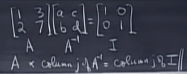
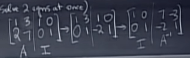
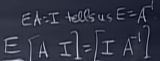
It’s a genius idea to arrive to the A inverse: also apply the elimination on the augmented matrix with identity matrix attached to the right side, eliminating until the left side matrix became identity. Why?

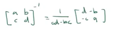
A square matrix that is not invertible is called singular or degenerate. A square matrix is singular if and only if its determinant is zero. How is determinant defined. It is to judge if a matrix component vectors are linear dependent or not, say if it is made up of [a, b, c, d], a/c = b/d means linear dependent, hence ad-bc=0, which is the determinant value. Find the invertible for a 2×2 matrix follows the rule as flip the diagonal a, d to d, a. then the other two leave as is, but add opposite sign in front.

Note if matrix A is not nxn square matrix, it is not invertible or it is singular. why? to reach to identity, identity matrix is square. To be more specific, if A is invertible, then the RREF form of A must be identity.

To solve matrix we can use row echelon form or reduced row echelon form RREF. RREF is unique. But REF could be sufficient for computation. The purpose of using REF is to deduce the solutions, esp. infinite many solutions scenario, for example

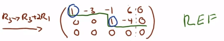
We can see column 2 and 4 are free since there is no leading 1s. So we can assume x2 = s and x4 = t, then from the second row, x3-4t = 0, x3 = 4t. Same way, we can get x1=3s+2t. In stead of finding a fixed vector [x1, x2, x3, x4] as a solution, in this case, it is[3s+2t, s, 4t, t].

The great invention of matrix is just a succinct form to express many equations. Ax=b, A is

and b is the x vector is the solution, b is the output vector, they live in different space. x in R^n, while b in R^m space. Note usually m is the row number and n is the column number if you count Matrix row x column. The way to carry out a matrix multiplication from its origin should be

Then we use row time column quick way to do this in head later on.

Ax=b vs Ax=0, or non-homogeneous vs homogeneous system solutions are both lines (assume A is [1 0, 2 0]), homogeneous solution goes through the origin.

How can I quickly find out the matrix of linear transformation? Experienced mathematicians or math teachers can just eyeball and write down the matrix, how do they do it?

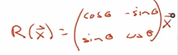
Let’s use an example to illustrate, say the transformation is to rotate counter clockwise theta degrees:

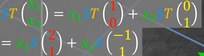
Note any vector x is expressed as the standard basis [e1, e2, … en] times vector component(in R), the transformation is expressed/manifested/understood as rendered on the whole standard basis system:

So any rotation by theta degree will cause the e1 basis to be cos(theta), sin(theta), e2 basis to be (-sin(theta), cos(theta). Hence plug in the above transformed form, we get

The flipping transformation would be

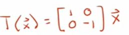
So the essence of this transformation is that it changes the component standard basis. from another angle – geometrically- we can see no matter how the transformation carries out, the instruction of forming the final vector is fixed.

Another trick that mathematicians do fast is apply elementary matrices in computation, for example

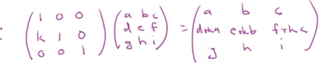
If you can read it as to manipulate the identity matrix to be k time first row and add to the second row forming this elementary matrix, the output then is also k time a, b, c adding to the second row d, e, f.

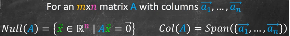
Again, the important concept of The Null Space & Column Space of a Matrix | Algebraically & Geometrically! after the matrix/transformation, all targets form a subspace, called “column space”, it lives in R^m, the codomain. It spans vectors of columns. Null space is the subspace, once transformed/matrixed, collapse to null/origin. It lives in R^n, the domain, to find null space, we just need to solve the homogeneous system.