Beta Distribution can be thought of as probability of probabilities, following up on previous example of good weather and bad weather, which is a Bernoulli Distribution, in 10 years, each year, the theta of having a good weather could vary, the probability could be uniform or various shaped between the boundary of 0 and 1. Beta distribution function is ideal to describe this probability of probability curve.

theta_weather = tfp.distributions.Beta(8.0,3.0)
weather = tfp.distributions.Bernoulli(probs=theta_weather.sample())
theta_weather.sample(100)
weather.sample(365)

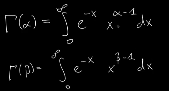
Above is the prelude knowledge about gamma distribution to help deduce the computation of beta distribution, particularly the normalization part. The process is math-heavy, but the output is

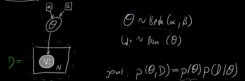
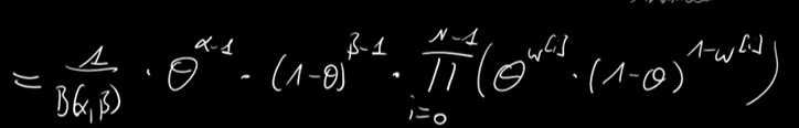
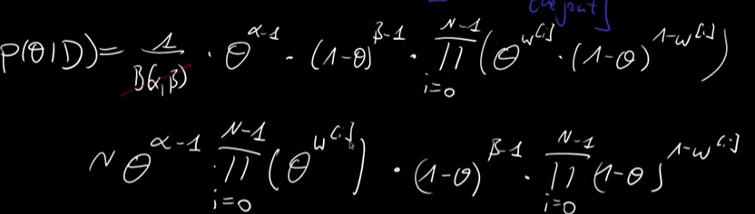
Knowing the conditional probability is always proportional to the joint probability, we can try to find the theta probability given a set of data D as below:

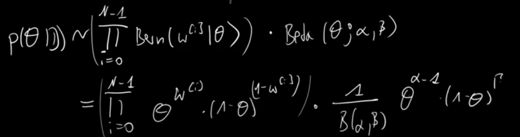
so end result is that we discover the posterior of  the Bernoulli model is also beta distribution. Again, the prior is Beta, the posterior is beta for model Bernoulli, this is called conjugate. It’s just the alpha beta parameters are alpha prime and beta prime accordingly.

Previously, we applied Maximum Likelihood Estimation calculation of theta, which turns out to be the mean of observations by analytical deduction and by gradient optimization. We’ll also apply Maximum A Posteriori Estimate (MAP) for Bernoulli here. What’s the difference? First, what is the MLE actually maximize? – it maximize the likelihood that the process described by the model produced the data that were actually observed. Hence the sample data here must be representative of true population, not corrupt.

P(theta|D) is the posterior, conditional probability, or probability of theta given/conditioned on the data D.

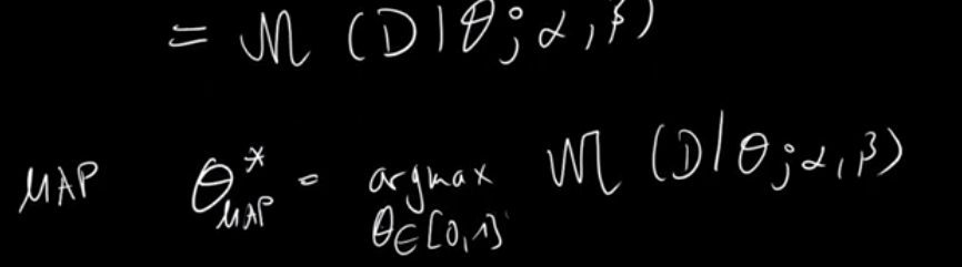
After a complex derivative calculation, reach

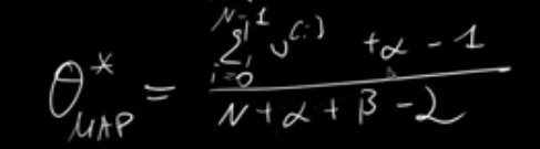
Comparing MLE and MAP, MAP usually could be better given parameter setting based on experts are valid.

It’s said repetitively that the marginal or the probability of dataset P(D) is very hard to calculate-intractable. Use above example, we can find P(D) by marginalizing the joint probability P(theta, D) over theta.

It’s impossible to find the anti-derivative/integral of above equation esp when the latent variable theta can go multiple.