“Bayesian statistics is a theory in the field of statistics based on the Bayesian interpretation of probability where probability expresses a degree of belief in an event. The degree of belief may be based on prior knowledge about the event, such as the results of previous experiments, or on personal beliefs about the event”. It’s an concept relative to Frequency statistics.

It is widely expressed by the Bayes Theorem:

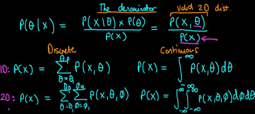
Note in nominator P(B | A) P(A) is equivalent to P(A, B), joint probability of A and B.

P(A) is the prior probability, without taking into any new data or new evidence, it could be based on blind belief, or more likely practiced by professional, based on prior experiments/accumulated data.

P(B) is the probability of the evidence, or new data. so if you had a collection of data composed of {A1, A2, … An}, then

or borrow from Ben Lambert:

Usually it’s hard to calculate, intractable but the nominator itself suffice the proportion estimate.

P(A | B) is the posterior probability, given new evidence B, the prior P(A) needs to be updated.

P(B | A) is the likelihood of B given A, interpreted as the probability of the evidence B given that A is true.

Use a simple model – Bayes Box as an example, if there are two balls, you don’t know how many are red, the task is to figure out the probability of two red balls, you can try to take out one ball, see if it’s red, then put it back and take out again to see if it’s red again.

In this simple case, the denominator, probability of tested data (two red balls) is computable to be 5/12. Let me describe each column here to make the concepts crystal clear:

R: Red balls in the bag can be 0, 1, 2, before the test, the prior belief is equal so

Pr(R): Probability of red balls is one third each

Pr(. .|R): Probability of two red balls given red balls in bag could be 0, 1, 2 respectively, adding them up the total does not necessary be 1, it’s a likelihood not probability per se.

Pr(R)xPr(. .|R): Joint likelihood, adding all the parts – joining part0, part1, part2 all together, it’s the denominator or marginal probability of two red balls(experimented data).

Pr(R|. .): Posterior probability, what’s the probability distribution given tested result is two red balls given the three scenarios, they will add up to 1, but if you are asked about the situation that there are two red balls, the specific posterior probability is 4/5 or 80%.

so if the example is flipping the coins 4 times, there are probability of 1, 2, 3, 4 heads, you can assume it’s equal chance or theta chance, by testing it out 10 time, 100 time, or 1000 times, the updated evidence/test results will yield a more and more accurate posterior probability distribution.

In real practice, purpose of using this Bayesian statistics theory, is to Maximum the likelihood estimation (MLE), or later on the notion of Maximum A Posteriori Estimate (MAP).  From the vantage point of Bayesian inference, MLE is a special case of maximum a posteriori estimation (MAP) that assumes a uniform prior distribution of the parameters.

The above example of picking two red balls from a bag containing two balls, the maximum likelihood seems to be the third scenario – there are two balls in bag -. Put it in another word, in this scenario, the likelihood of observing the experimental data – picking two red balls in a row – is the maximum.

Usually in real practice, we need to have a model for prior estimation and then use this MLE approach to evaluate if the model, and the parameters of the model makes the observed data mostly likely.