In previous blog – Probability Density Functions(PDF)_Beta Distribution, MLE and MAP were mentioned about maximizing the likelihood of P(theta) given the observed data(evidence). It is part of the broader concept called EM(expectation Maximization).

Note P(theta) = P(R) in that two red balls selected out of a bag of two balls instance. Always be very clear of what these symbols mean!

Dr.Richard Xu 徐亦达 has a very clear playlist on EM, which I referenced. ritvikmath‘s EM explanation is superior.

Jensen’s inequality will be used to deduce variational inference. What is Jensen’s inequality? from wiki graph below, any point on the convex (function f) can be expressed as f(tx1 + (1-t)x2) where t varies between 0 and 1; while the line formed by the intersection can be expressed as tf(x1) + (1-t)f(x2).

Argmax is needed to explain. arguments of the maxima (abbreviated arg max or argmax) are the points, or elements, of the domain of some function at which the function values are maximized. It returns the value x that maximize the function f(x).

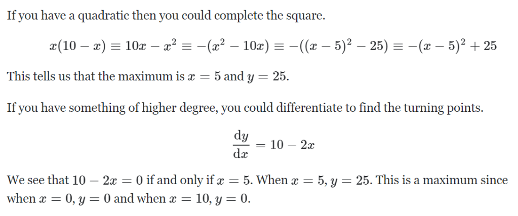
The above explains how it is computed using an example.

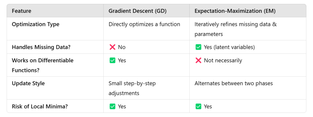
This approach is unlike other methods such as gradient descent, conjugate gradient, or variants of the Gauss–Newton algorithm. Unlike EM, such methods typically require the evaluation of first and/or second derivatives of the likelihood function.

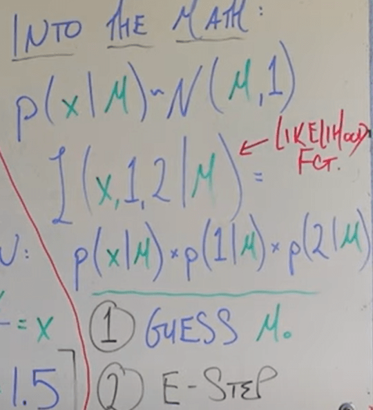
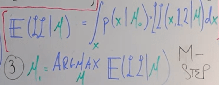
It’s worth emphasizing that I was confused about whether the miu is actually maximized or miu is just the value that returns the maximized probability of something. When Dr.Richard Xu constantly say ‘maximizing miu’, he is right in the sense when you find the value E, it is the maximum likely to be expected in a probability distribution. The only difference is that if you get a easy case, given PDF and value Xs, you can do summation/integral to compute easily; when data Xs is also missing, and you are asked to find Xs, an iterative argmax is used here to find the E.

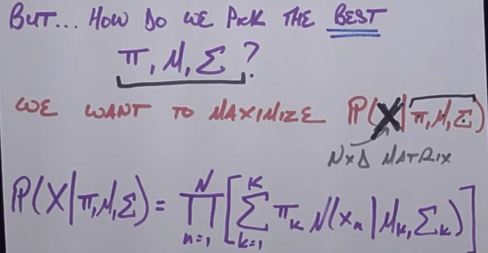
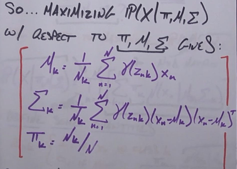
Below we go through GMM Gaussian Mixture Model to compute the E:

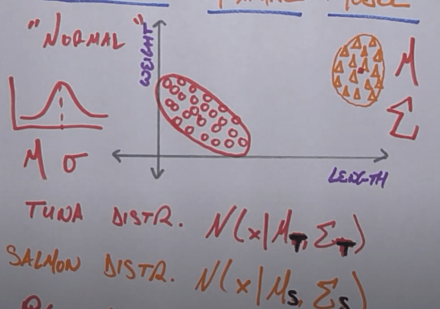
in this example, there data points on fish’s weight and length, seems they form two clusters both following Gaussian distribution, we need to find the parameters of the two Gaussian and another parameter pie denoting the probability of being included in Tuna or Salmon Gaussian.

use coin flipping as an example in simplest form: you don’t know the probability of coin flipping to head or tail; you flipped twice each 5 times. in the first trial, you got 3 heads 2 tails, second trial is unknown. Now apply EM to “guess” out the probability of this coin and second trial maximum likely output.

first, assume theta, the intrinsic probability of this coin as 0.5, then based on this argument, derive per maximum likelihood, the second trial should have 5*0.5 heads;

second, recompute the theta given the data: (3+2.5)/10 = 0.55, higher than initial assumption of 0.5, hence update theta = 0.55,

do the same step first and step second, this time the new heads number in second trial is 0.55*5, and updated theta = 3+0.55*5/10=0.575,

do the same, theta = 0.5875, until it reaches 0.6, when the assumed theta is consistent with the mostly likely trial 2 data: 0.6*5=3, 3+3/10=0.6, we say it converges!