By applying this frozen lake toy example, we can pick up the math beneath it.

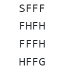
The game is to explore and try jump on frozen lake made up of holes and safe ice until reach the goal.

Then we can start coding to grasp Reinforcement Learning math.

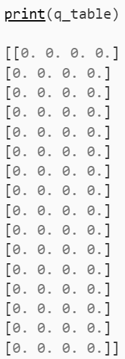
First, to create the Q-table,  number of rows is the size of the state space in the environment, in this case it’s 16 state space; the number of columns is equivalent to the size of the action space, in this case, only 4 moves/actions, up down left right.

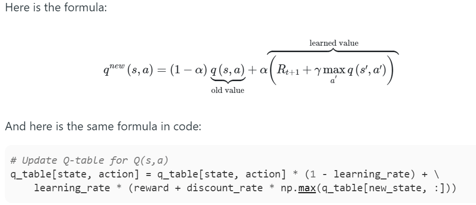
The math essence here is to update the Q-value table

Along the way, the exploration rate needs to be updated too so the agent doesn’t exploring too much and get stuck in cycle.

exploration_rate = 1; max_exploration_rate = 1; min_exploration_rate = 0.01; exploration_decay_rate = 0.01

# Exploration rate decay exploration_rate = min_exploration_rate + \ (max_exploration_rate – min_exploration_rate) * np.exp(-exploration_decay_rate*episode)

All the codes are here

# Reinforcement Learning Q learning 
import gym
import random
import time
import numpy as np


env = gym.make("FrozenLake-v1")

action_space_size = env.action_space.n
state_space_size = env.observation_space.n

q_table = np.zeros((state_space_size, action_space_size))
num_episodes = 10000
max_steps_per_episode = 100

learning_rate = 0.1
discount_rate = 0.99

exploration_rate = 1
max_exploration_rate = 1
min_exploration_rate = 0.01
exploration_decay_rate = 0.01

rewards_all_episodes = []
# Q-learning algorithm
for episode in range(num_episodes):
    # initialize new episode params
    state = env.reset()
    done = False
    rewards_current_episode = 0

    for step in range(max_steps_per_episode): 
        # Exploration-exploitation trade-off
        exploration_rate_threshold = random.uniform(0,1)
        # Take new action
        if exploration_rate_threshold > exploration_rate:
            action = np.argmax(q_table[state, :])
        else:
            action = env.action_space.sample()    
        new_state, reward, done, info = env.step(action)
        # Update Q-table
        q_table[state, action] = q_table[state, action] * (1 - learning_rate) + \
            learning_rate * (reward + discount_rate * np.max(q_table[new_state, :]))
        # Set new state
        state = new_state
        # Add new reward 
        rewards_current_episode += reward 

        if done == True:
            break
               

    # Exploration rate decay   
    exploration_rate = min_exploration_rate + \
        (max_exploration_rate - min_exploration_rate) * np.exp(-exploration_decay_rate*episode)
    rewards_all_episodes.append(rewards_current_episode)

    # Calculate and print 
    rewards_per_thousand_episodes = np.split(np.array(rewards_all_episodes), num_episodes/1000)
    count = 1000
    print("******Average reward per thousand episodes*****\n")
    for r in rewards_per_thousand_episodes:
        print(count, ": ", str(sum(r/1000)))
        count += 1000
    # Print updated Q-table
    print("\n\n***Q-table***\n")
    print(q_table)

Q-learning is a model-free reinforcement learning algorithm that learns the optimal action-selection policy in an unknown environment by trial and error. Comparing it to A* is a search algorithm used for shortest path finding in a known environment.

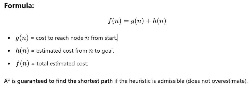
magine a robot navigating a maze:

• A*: The robot already has a map of the maze and uses a heuristic to find the shortest path efficiently.
• Q-Learning: The robot starts without knowing the maze. It explores, tries different paths, learns from rewards, and eventually figures out the best way over time.

🔹 A* is for optimal pathfinding in a known world, Q-learning is for learning optimal actions in an unknown world.