The Kalman filter, famous from its use in the Apollo moon missions, is now widely used in areas like autonomous driving and robotics. It’s great at dealing with data that has a lot of Gaussian distributed ‘noise’ and can predict how things might change over time, which is useful for stock price prediction.
I’m planning to use a basic Kalman filter to predict prices for two stocks – FactSet and Tesla. Since Tesla’s price is a lot more volatile, I’ll need to adjust the covariance parameter accordingly.
Stock prices movement is not stationary, so I’m going to work with daily price returns instead. To account for the whole market movement, i.e. beta effect, I’ll use ‘excess return’, which is the daily return of the target stock minus the daily return of the S&P 500. This excess return is an Autoregressive Series rather than a random walk, of which the variance increases over time and is non-stationary.
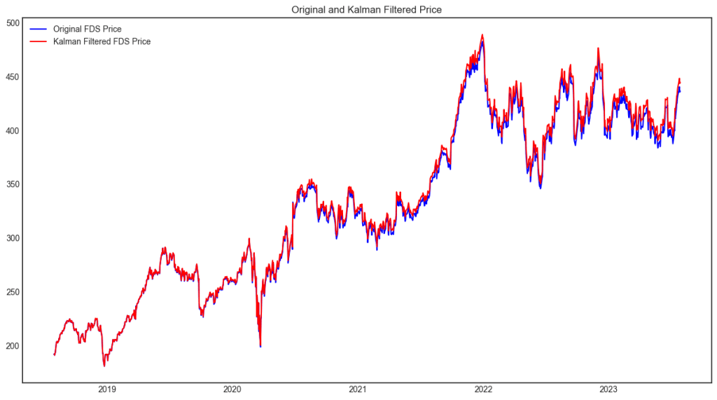
So for FDS-US, I set parameter as
kf = KalmanFilter(transition_matrices=[1],
                  observation_matrices=[1],
                  initial_state_mean=0,
                  initial_state_covariance=10,
                  observation_covariance=1,
                  transition_covariance=10)
and output is as below:
Tesla is notoriously volatile, if I apply the same parameter as FDS, the prediciton is horrible, however, adjusting initial_state_covariance and transition_covariance=100, the matching/predicting is remarkable:

It’s intriguing to apply this basic form of the Kalman filter by making simple assumptions about the noise and factors affecting stock price movements. In reality, these dynamics are incredibly complex, which limits the practical use of this approach. Adjusting the parameters for these models requires significant mathematical finesse, for which I plan to apply EM algorithm to learn the parameters automatically next time.
The full codes are:
# try Kalman filter on FDS-US analysis
pip install pykalman
pip install pandas-datareader
import numpy as np
import pandas as pd
import yfinance as yf
from pykalman import KalmanFilter
import matplotlib.pyplot as plt
from datetime import datetime, timedelta

# Define the start and end dates
end = datetime.now()
start = end - timedelta(days=5*365)

# Fetch the data for FDS and S&P 500
fds_data = yf.download('FDS', start=start, end=end)
sp500_data = yf.download('^GSPC', start=start, end=end)

# Compute the daily returns
fds_returns = fds_data['Adj Close'].pct_change().dropna()
sp500_returns = sp500_data['Adj Close'].pct_change().dropna()

# Compute the excess returns
excess_returns = fds_returns - sp500_returns

# Create a Kalman Filter model
kf = KalmanFilter(transition_matrices=[1],
                  observation_matrices=[1],
                  initial_state_mean=0,
                  initial_state_covariance=10,
                  observation_covariance=1,
                  transition_covariance=10)

# Use the observed values of the excess returns to get a filtered estimate
state_means, _ = kf.filter(excess_returns.values)

# Convert the state means to a pandas series, to put dates back
state_means = pd.Series(state_means.flatten(), index=excess_returns.index)

# Plot original data and estimated mean
# plt.figure(figsize=(15,8))
# orig = plt.plot(excess_returns, color='blue', label='Original Excess Returns')
# mean = plt.plot(state_means, color='red', label='Kalman Estimate Mean')
# plt.legend(loc='best')
# plt.title('Kalman Filter estimate of average')
# plt.show()

# Add the excess returns to the benchmark returns to get filtered returns
filtered_returns = state_means + sp500_returns

# Now, compute the filtered price series from the filtered returns and the first stock price
first_price = fds_data['Adj Close'][0]
filtered_prices = (filtered_returns + 1).cumprod() * first_price

# Plot original and filtered price data
plt.figure(figsize=(15,8))
orig_price = plt.plot(fds_data['Adj Close'], color='blue', label='Original FDS Price')
filtered_price = plt.plot(filtered_prices, color='red', label='Kalman Filtered FDS Price')
plt.legend(loc='best')
plt.title('Original and Kalman Filtered Price')
plt.show()
