On top of discrete scenario, further on to investigate the continuous, we want the inner product to realize the same – single out the coefficient pointing to the specific state, 2.71 in below case.

ok, what is Dirac delta function, it was told to be a big spike but the integral of which at that point = 1. The genius Dirac makes use of Dirac delta function in a way that when delta(x), it blow up to infinity,

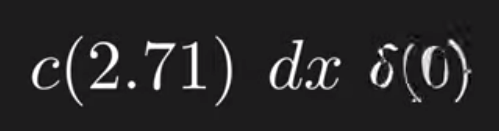
hence d(x)delta(0) gets canceled out the right part = 1, so we get c(2.71) to make math equation tied to physics needs. It’s fun to dig deeper as the infinity integral =1 just seems skeptical, we found Gaussian equation can mimic/equate Dirac delta when alpha goes big, so is the following though, the following oscillates not one pure spike:

to deal with above paradox, Brandon stated the right definition of delta is

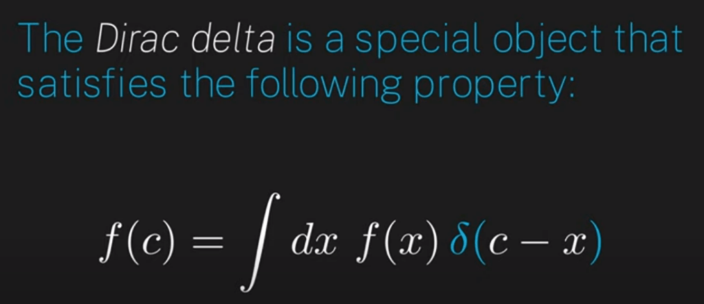
Now let’s put it to application of QM for continouse property calculation:

Next introduce the concept of row matrices, dual vector and dual space, the Lphi is a linear functional that acts on vector v is equivalent to taking the inner product of two wave function/quant states phi and v:

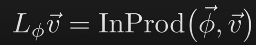
Thus, the Diract notation/bra-ket notation.

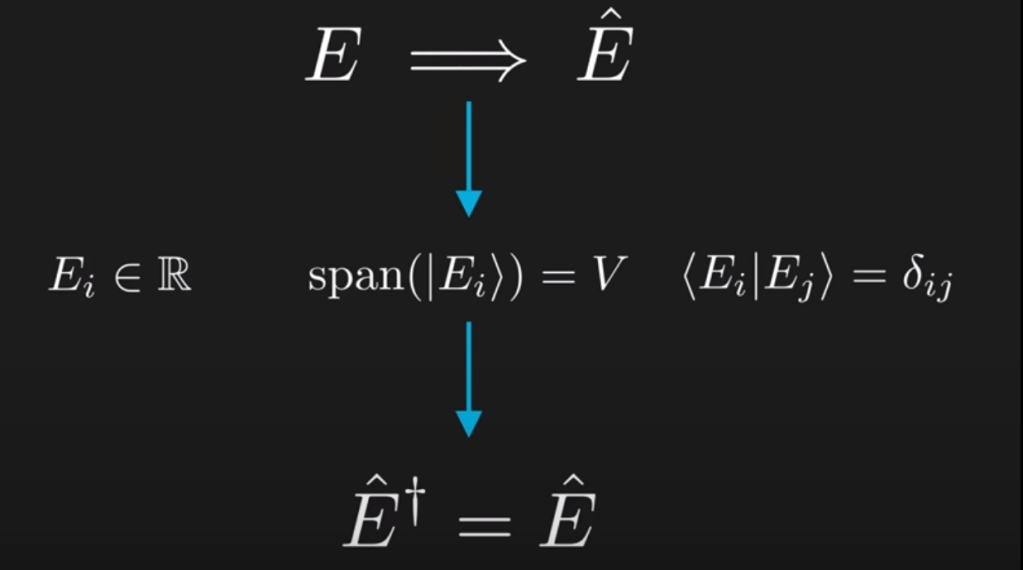
All obersevables are formed by orthonormal eigenbasis. Next we need to figure out why these observables have to be Hermitian. in stead of being told, we need to reason it out.

Brandon is brilliant in showing what Hermitian in regular operator operating:

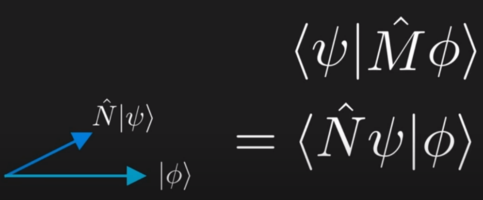
We try to figure out if there is such a N operator that acts on sai leading to same output. We define it as Hermitian adjoint if it’s true, and also write it as M+:

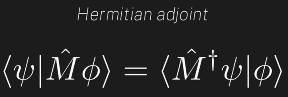
There are some properties of Hermitian adjoint, that’s easy to prove, particularly.

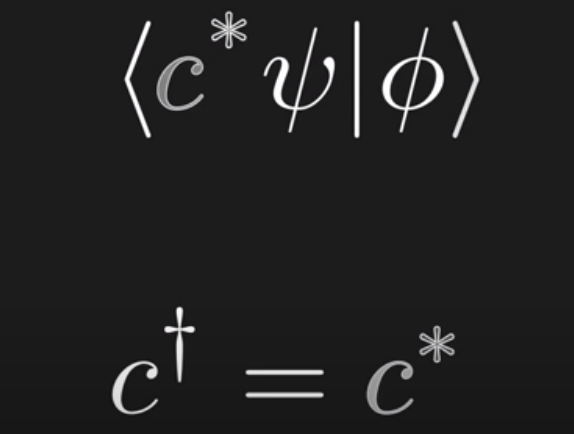
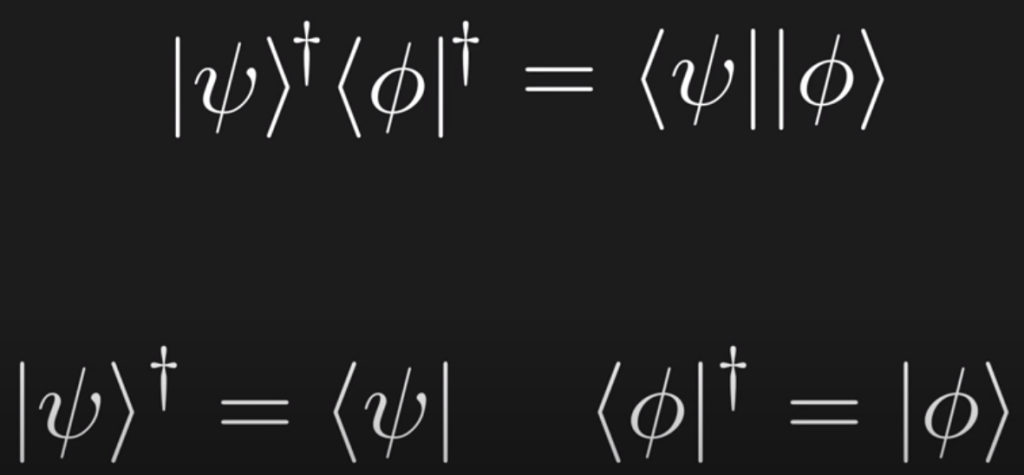
Further, even we’ve discussing Hermitian adjoint on the base of matrix/operator, we can also ask the question, what is the Hermitian of ket? It’s actually mathematically derivable that the Hermitian of bra is ket, and the Hermitian of ket is bra:

Why Hermitian adjoint is so useful in QM?

Then proves that The Hermitian of the observable is the observable itself. They are called Hermitian operators.

In summary, Brandon uses the physics intuition, and grasp the mathematical tool to apply

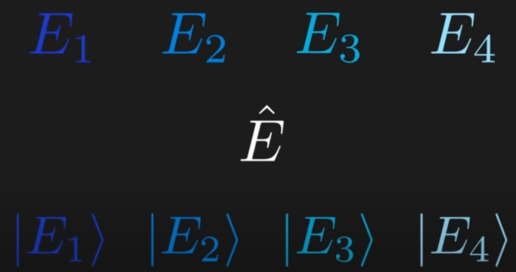
Born Rule, which bothered me a great deal a year earlier. Note the way to interpret is that the sai state/ket project on the bra E4:

Brandon, instead of just throwing you the Born rule, which is very confusing and seems from thin air, he took great deal efforts to mathematically derived or proved the square of coefficients are the probability-Born rule.

Note first row E1,E2 are the eigen values for E hat, the quantum state, the third row is the eigen vectors.

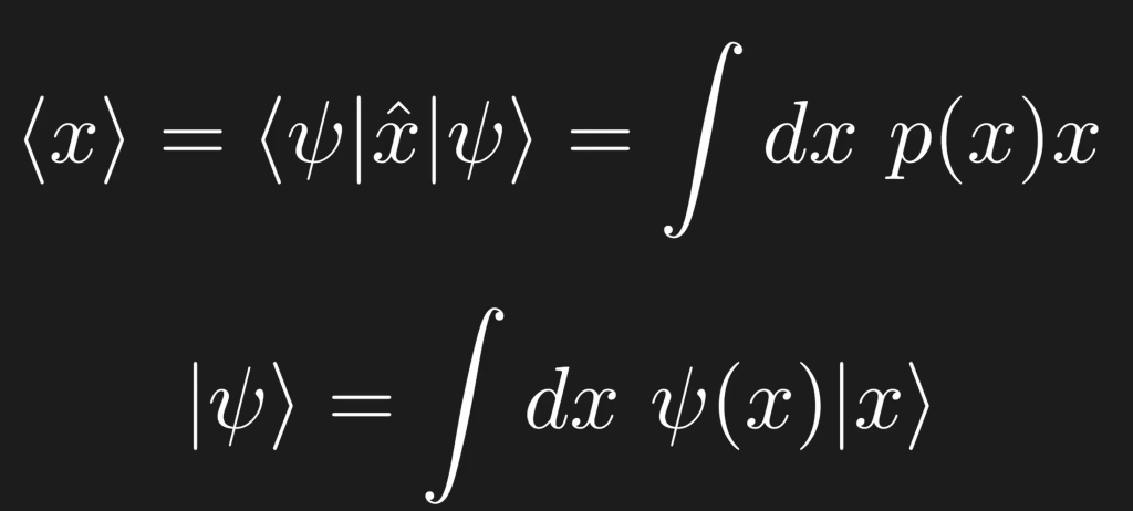
Adding on the fundamental mind behind Brandon is that to look at Quantum state represented by sai ket as a combination of various quantities such as discrete energy, angular momentum, and continuous position x, in the case of continuous position x, summation became integral, hence

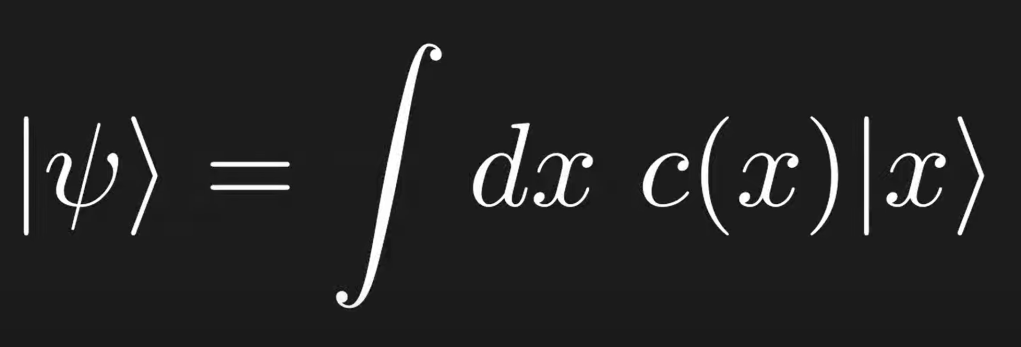
later on we replace the coefficient function c(x) with wave function, also well known that the wavefunction is tied to the probability in QM. see below Schrodinger Equation in describing the wavefunction:

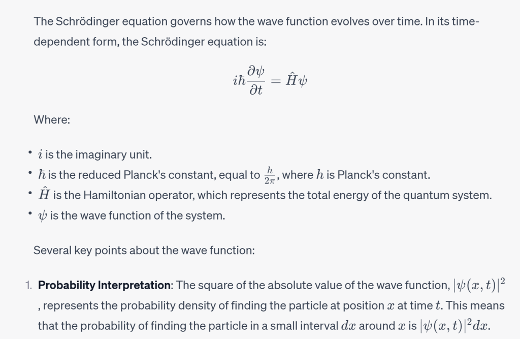
Now we need to bring in the key idea what this wave function represents is just the probability measurement or coefficient. But how? How to make this thinking leap from coefficient x to wave function x?

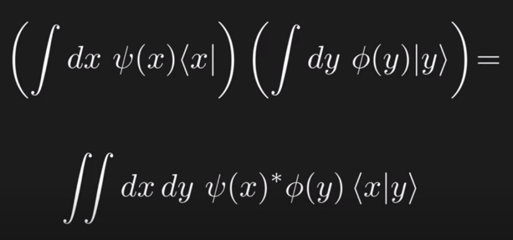
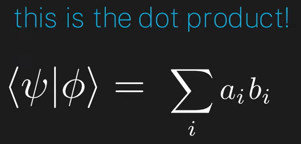
It’s due to our previous knowledge about dot product between a specific state(be it energy or position) with the sai wave function, we single out only the term on that specific state amplitude:

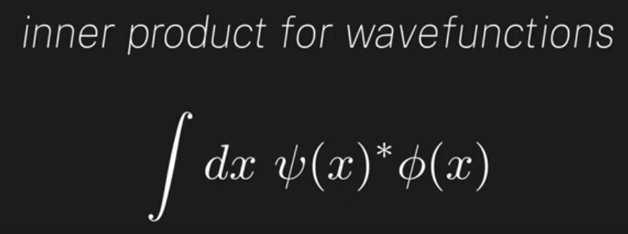
We can then deduce the below dot product between two wavefunctions is exact consistent with the traditional dot product definition for two vectors.

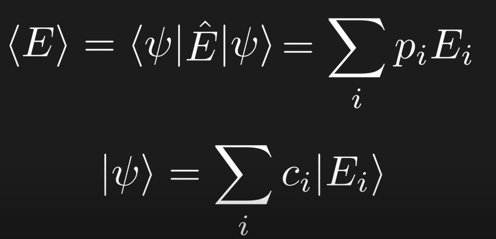
leading to Born’s rule, which was a big puzzle for a long time, then also puzzled me long time is why expected value of E is the sanwidge structure:

And if the quantity to measure is continuous say position