Thera are two main approaches for optimal portfolio selection are considered in the literature. One is based on a straightforward risk-reward trade-off analysis. The other is based on the portfolio manager expected utility preferences.

First approach pioneered by Markowitz, the Markowitz portfolio optimization model is considered as the corner-stone of the modern portfolio theory. It became popular as the Mean-variance (M-V) portfolio analysis — a traditional theoretical approach utilized almost everywhere in modern financial world. The M-V analysis results in a portfolio which is a preferred investor choice if it has higher expected (mean) return and lower variance.

The second approach is the expected utility optimization which follows some axiomatic preferences. It dates back to the work of Neumann and Morgenstern. it can be demonstrated that there is consistency with a smaller class of investors — those with quadratic utility functions or with utility functions which can be sufficiently well approximated by quadratic utilities.

Bit more details on mean-ETL portfolio optimization model (Section 4).

The utility type of Markowitz optimization

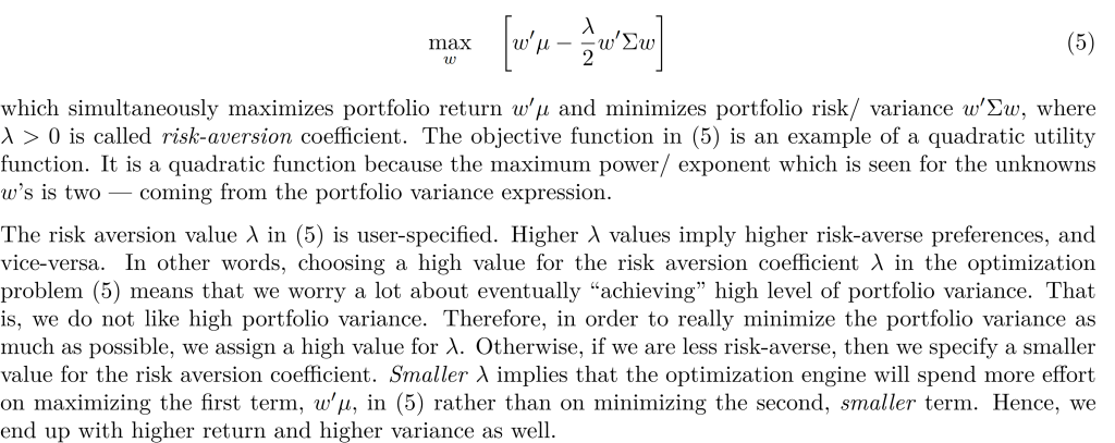
The lambda (λ) in utility-type Markowitz portfolio optimization and the lambda in L1 and L2 regularization are conceptually different:

1. In Markowitz Portfolio Optimization: Lambda (λ) represents the risk aversion coefficient. It quantifies how much risk an investor is willing to take. A higher lambda implies more risk aversion (preference for lower risk), and the optimization focuses more on minimizing risk relative to the expected return.
2. In L1 and L2 Regularization: Lambda is the regularization parameter. It controls the strength of the regularization. In L1 regularization (Lasso), it determines how many features will be set to zero (sparsity), while in L2 regularization (Ridge), it controls the shrinking of the coefficients to reduce overfitting.

Convex programming is a subclass of mathematical optimization problems where the objective function is convex and the constraints form a convex set. This means that any local minimum is also a global minimum, simplifying the optimization process.

Quadratic programming, a specific type of convex programming, involves an objective function that is a quadratic function of the variables and linear constraints. While all quadratic programming problems are convex (assuming the quadratic function is convex), not all convex programming problems are quadratic, as the objective function in convex programming can be any convex function, not limited to quadratic forms.

Solvers for convex functions

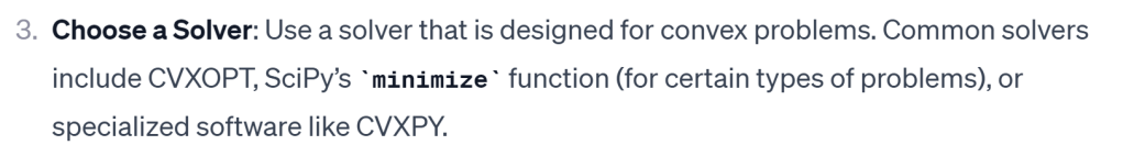
The mathematics behind convex optimization solvers generally involve iterative algorithms to find the minimum of a convex function over a convex set. Common methods include:

• Gradient Descent: Used in differentiable problems. It iteratively moves towards the minimum by taking steps proportional to the negative of the gradient (or approximate gradient) of the function.
• Interior-Point Methods: These are efficient for large-scale convex problems. They traverse the interior of the feasible region and exploit its curvature to make rapid progress towards the optimum.
• Simplex Method: Primarily used for linear programming. It moves along the edges of the feasible region to find the best vertex that minimizes the objective function.
• Sequential Quadratic Programming: Used for nonlinear problems. It approximates the problem by a quadratic programming problem at each iteration.

Each of these methods leverages the properties of convex functions, such as the fact that any local minimum is also a global minimum, to efficiently find the optimal solution.