The Poincaré map, named after Henri Poincaré, is a significant concept in the study of dynamical systems. It’s a method used to simplify the understanding of complex, multidimensional systems by reducing them to a lower-dimensional space.

How It Works: Imagine a multidimensional space where a dynamical system evolves over time. The Poincaré map takes a ‘slice’ of this space at regular intervals. This ‘slice’ is a lower-dimensional subspace, like a plane in a three-dimensional space. By observing where the trajectories of the system intersect this plane, the map provides insights into the system’s behavior over time.

Let’s consider a classic example of a Poincaré map in action: the analysis of a simple pendulum.

# poincare map

import numpy as np

import matplotlib.pyplot as plt

from scipy.integrate import solve_ivp



# Constants for the pendulum

b = 0.5  # Damping coefficient

c = 1.0  # Proportional to gravitational force and pendulum length



# Differential equations for the pendulum

def pendulum_equations(t, y):

    theta, omega = y

    dtheta_dt = omega

    domega_dt = -b * omega - c * np.sin(theta)

    return [dtheta_dt, domega_dt]



# Initial conditions: [theta0, omega0]

initial_conditions = [np.pi / 4, 0]



# Time span for the simulation

t_span = [0, 100]

t_eval = np.linspace(t_span[0], t_span[1], 1000)



# Solve the differential equation

solution = solve_ivp(pendulum_equations, t_span, initial_conditions, t_eval=t_eval)



# Extracting theta and omega from the solution

theta = solution.y[0]

omega = solution.y[1]



# Poincaré map: Sampling points at regular time intervals

sampling_interval = 2 * np.pi / np.sqrt(c)  # Approximate period of the pendulum

sampling_times = np.arange(t_span[0], t_span[1], sampling_interval)

sampling_indices = np.searchsorted(t_eval, sampling_times)

poincare_theta = theta[sampling_indices]

poincare_omega = omega[sampling_indices]



# Plotting the Poincaré map

plt.figure(figsize=(8, 6))

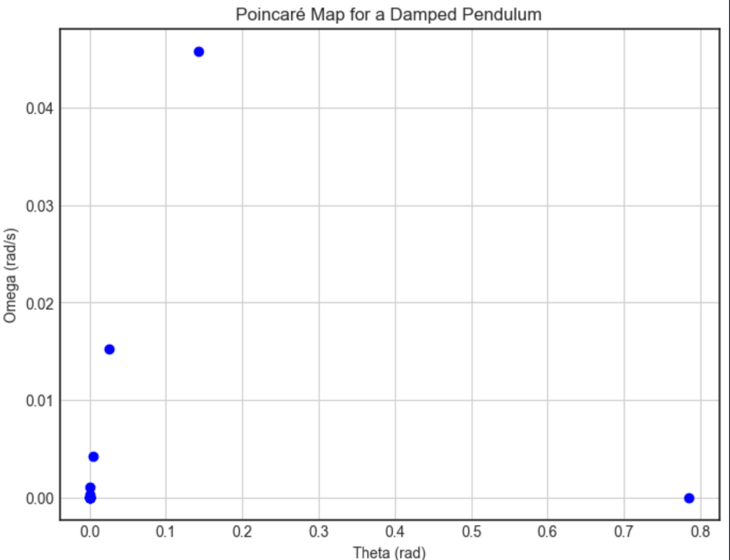
plt.scatter(poincare_theta, poincare_omega, color='blue')

plt.title('Poincaré Map for a Damped Pendulum')

plt.xlabel('Theta (rad)')

plt.ylabel('Omega (rad/s)')

plt.grid(True)

plt.show()