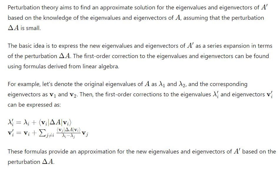
First, need to apply a simple Matrix example to learn what perturb technique is:

Sure, let’s consider a simple 2×2 matrix example to explain perturbation theory.

Let’s say we have the following original matrix ( A ):

[ A = \begin{bmatrix} a & b \ c & d \end{bmatrix} ]

Now, let’s say we have a small perturbation matrix ( \Delta A ) that we add to ( A ):

[ \Delta A = \begin{bmatrix} \Delta a & \Delta b \ \Delta c & \Delta d \end{bmatrix} ]

So, the new matrix ( A’ ) becomes:

[ A’ = A + \Delta A = \begin{bmatrix} a + \Delta a & b + \Delta b \ c + \Delta c & d + \Delta d \end{bmatrix} ]

In more complex systems, perturbation theory can be applied iteratively to find higher-order corrections to the eigenvalues and eigenvectors, providing increasingly accurate approximations as needed.

How is it derived? skipped next time

In quantum field theory (QFT), the ϕ4 theory describes scalar fields interacting through a quartic potential. In ϕ4 theory, the Lagrangian density is given by:

sidenote: free chatGPT is the best in showing math formulas, claude, perplexity or chatGPT plus all failed.