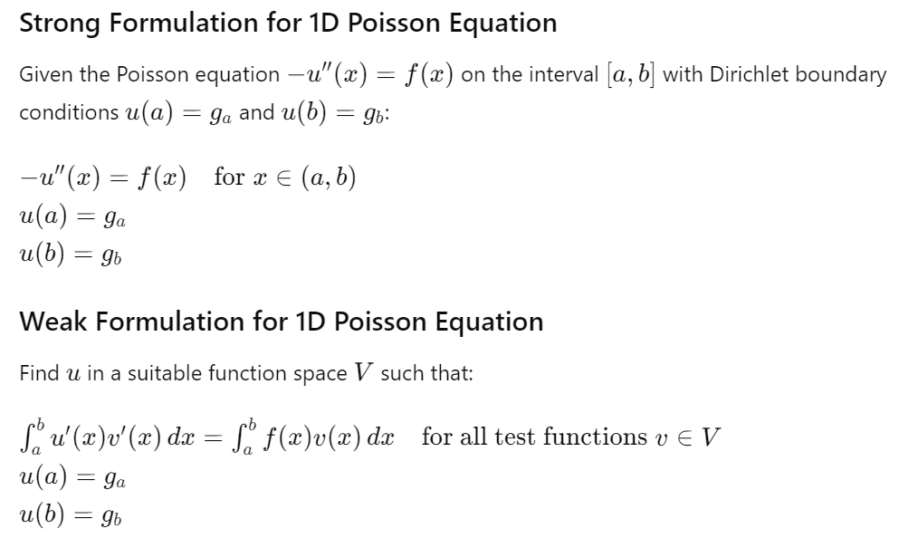
Strong Formulation: Directly involves the original differential equations and boundary conditions that must be satisfied exactly at every point in the domain. Weak Formulation: Transforms the differential equation into an integral form, typically using test functions and integration by parts, allowing for approximate solutions within a finite-dimensional subspace.
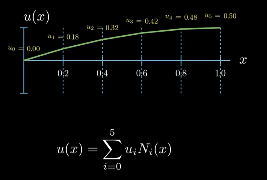
Now introduce the finite discrete element method idea
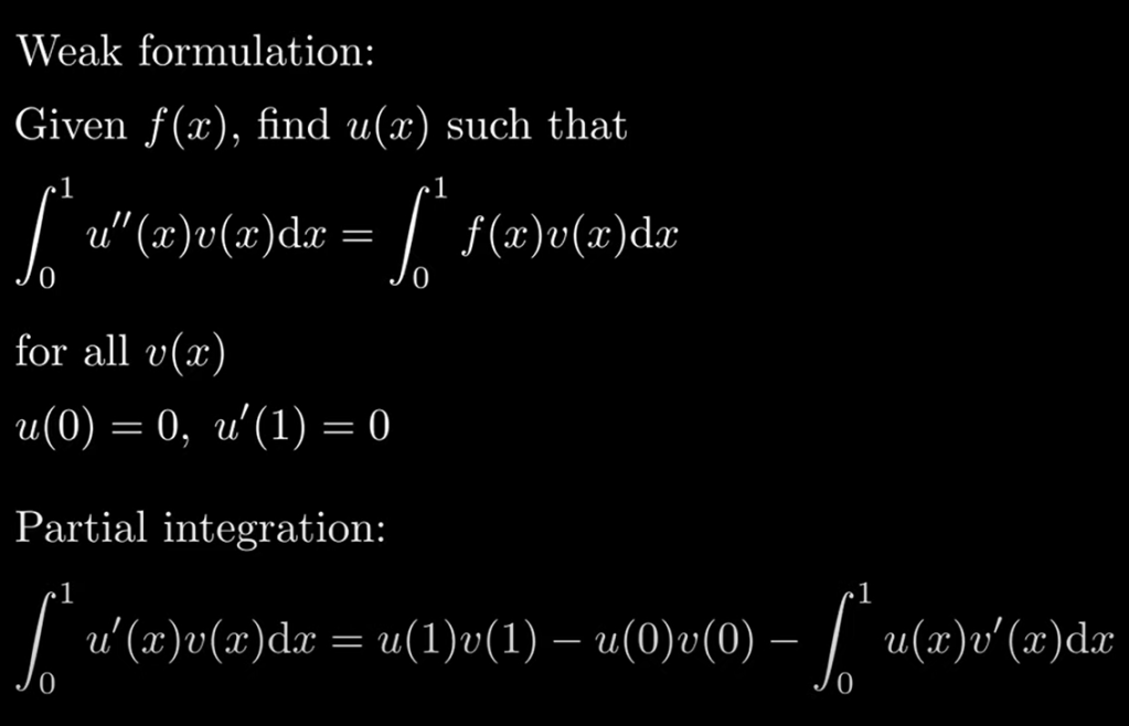
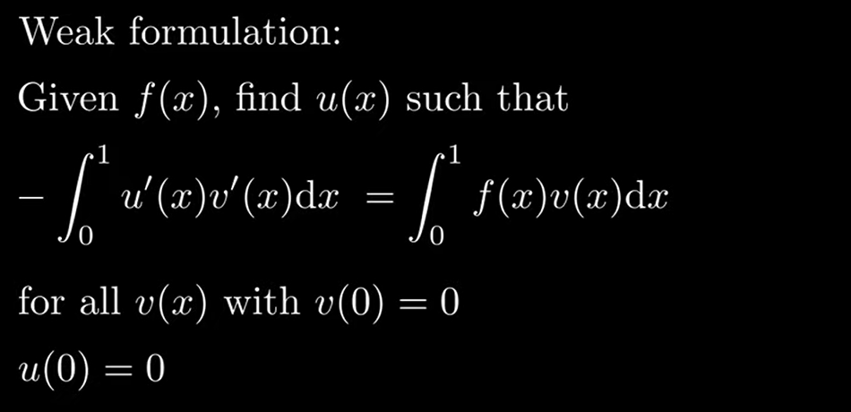
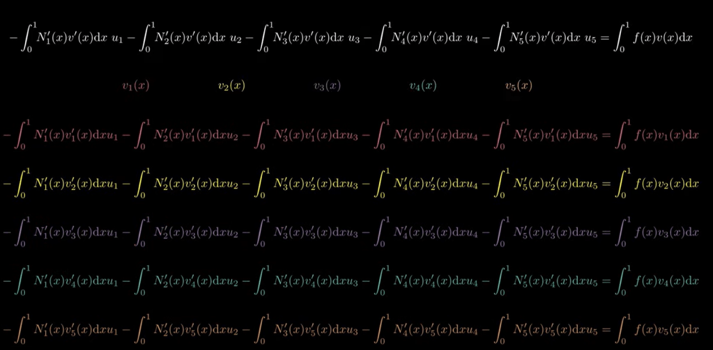
But how to use it in numerical analysis, let’s derive from
Now replace it with N function dissected to elements:
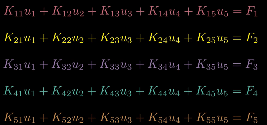
this is the genius work by computational modeling expert.
Sample codes applying FEM to simulate a function
# FEM sample codes
import numpy as np
import scipy.sparse as sp
import scipy.sparse.linalg as spla

# Parameters
L = 1       # Length of the domain
N = 10      # Number of elements
h = L / N   # Element size

# Source function
def f(x):
    return np.sin(np.pi * x)

# Grid points
x = np.linspace(0, L, N + 1)

# Stiffness matrix and load vector
K = sp.lil_matrix((N + 1, N + 1))
F = np.zeros(N + 1)

# Assemble the stiffness matrix and load vector
for i in range(1, N):
    K[i, i - 1] = 1 / h
    K[i, i] = -2 / h
    K[i, i + 1] = 1 / h
    F[i] = f(x[i]) * h

# Apply boundary conditions (Dirichlet boundary conditions u(0) = u(L) = 0)
K[0, 0] = K[N, N] = 1
K[0, 1] = K[N, N - 1] = 0
F[0] = F[N] = 0

# Convert to CSR format for efficient solving
K_csr = K.tocsr()

# Solve the linear system Ku = F
u = spla.spsolve(K_csr, F)

# Actual solution
u_actual = -(1 / np.pi**2) * np.sin(np.pi * x)

# Plot the solutions
plt.plot(x, u, label='FEM Solution', marker='o')
plt.plot(x, u_actual, label='Actual Solution', linestyle='--')
plt.xlabel('x')
plt.ylabel('u(x)')
plt.legend()
plt.title('FEM Solution vs Actual Solution for Poisson Equation')
plt.show()

