Follow the github page by Dr. Karparthy: https://github.com/karpathy/build-nanogpt and youtube: https://www.youtube.com/watch?v=l8pRSuU81PU&list=PLAqhIrjkxbuWI23v9cThsA9GvCAUhRvKZ&t=1175s, the whole series is worth deep diving hence here it is, right from the very beginning.

First, basics by Andrej, he illustrated how manually applied micro level backward propagation in the first great video: macrograd!

with these two simple py file, engine.py and nn.py, Andrej explained perfectly what activation function, forward propagation, backward propagation, regularization are. And certainly great deal of his coding arts. The key is to compute grad or gradient.

It’s computed numerically or analytically? apparently it is numerically in actual life, the equation is not given, and hence in NN, there is this important concept of “learning rate” which basically is the stride width set up in doing numerical iteration.

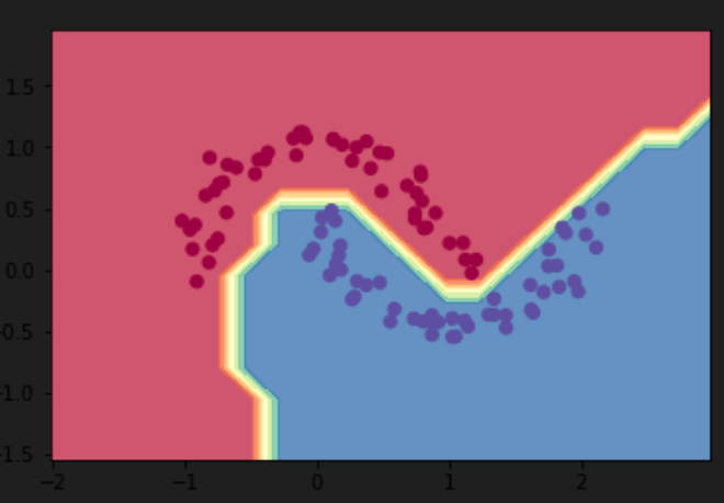
using the example in his latest micrograd repo, to learn the boundary line to seperate the two blocks of dots, his MLP accomplished the goal by setting up 2 layers of 16-component neurons, Input layer: 2 inputs

First hidden layer: 16 ReLU neurons (16 * 2 weights + 16 biases = 48 parameters)

Second hidden layer: 16 ReLU neurons (16 * 16 weights + 16 biases = 272 parameters)

Output layer: 1 Linear neuron (1 * 16 weights + 1 bias = 17 parameters)

The output line is f(x1, x2), hence the initial layer is two.

the choice of two layers with 16 neurons each is somewhat arbitrary, which can be experimented using test data.

To grasp, I will write down every bit of code and its design step by step:

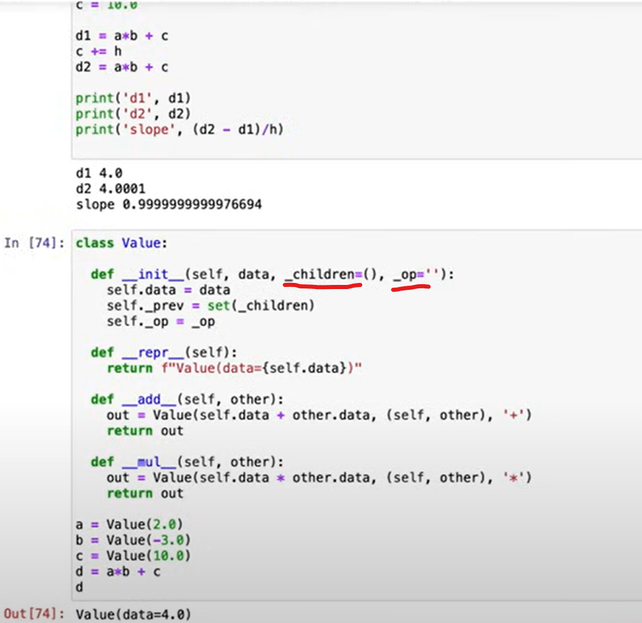
first, to deal with nn, tensor is inevitable, but we start from Value class to handle the simplest form of tensor, to store single scalar value and its gradient. in Value initial constructor, _backward is initialized to lambda: None as a placeholder to ensure the object is valid even if backward propagation is not yet defined.

    def __add__(self, other):
        other = other if isinstance(other, Value) else Value(other)
        out = Value(self.data + other.data, (self, other), '+')

        def _backward():
            self.grad += out.grad
            other.grad += out.grad
        out._backward = _backward

        return out

second, in this function under function, note the out is returned, then you can call out.backward, no parenthesis to get the grad computation done.

    def relu(self):
        out = Value(0 if self.data < 0 else self.data, (self,), 'ReLU')

        def _backward():
            self.grad += (out.data > 0) * out.grad
        out._backward = _backward

        return out

in this Relu function, note out.data > 0 condition, is a condition, but it returns a Boolean result (True/False) or a Boolean array.

    def __repr__(self):
        return f"Value(data={self.data}, grad={self.grad})"

repr as interpretation.

    def backward(self):

        # topological order all of the children in the graph
        topo = []
        visited = set()
        def build_topo(v):
            if v not in visited:
                visited.add(v)
                for child in v._prev:
                    build_topo(child)
                topo.append(v)
        build_topo(self)

        # go one variable at a time and apply the chain rule to get its gradient
        self.grad = 1
        for v in reversed(topo):
            v._backward()

The entire backward function taking topological sorting recursively.

class Module:

    def zero_grad(self):
        for p in self.parameters():
            p.grad = 0

    def parameters(self):
        return []

class Neuron(Module):

The Module class acts as a base class for all components (neurons, layers, networks). By defining standard methods like parameters and zero_grad, it ensures that all derived classes adhere to a consistent interface. provides a common foundation that simplifies working with increasingly complex models. As you build deeper networks with multiple layers.

class Layer(Module):

    def __init__(self, nin, nout, **kwargs):
        self.neurons = [Neuron(nin, **kwargs) for _ in range(nout)]

    def __call__(self, x):
        out = [n(x) for n in self.neurons]
        return out[0] if len(out) == 1 else out

x is a list, same as the input in Neuron class, for example, layer = Layer(nin=3, nout=2) # Layer with 2 neurons x = [1.0, 2.0, 3.0] # Example input output = layer(x) # x is passed to each of the 2 neurons, and their outputs are collected into a list. # Output will be a list with 2 elements, one from each neuron.

class MLP(Module):

    def __init__(self, nin, nouts):
        sz = [nin] + nouts
        self.layers = [Layer(sz[i], sz[i+1], nonlin=i!=len(nouts)-1) for i in range(len(nouts))]

If i is not the last layer, the condition i != len(nouts)-1 is True, so nonlin=True.

Next apply the make moon datasets to test it out.

X, y = make_moons(n_samples=100, noise=0.1) print(X.shape) # Output: (100, 2) print(X.shape[0]) # Output: 100 (number of samples) print(X.shape[1]) # Output: 2 (number of features)

inputs = [list(map(Value, xrow)) for xrow in Xb]
scores = list(map(model, inputs))
model = MLP(2, [16, 16, 1]) # 2-layer neural network

Xb = [[1.2, 3.4], [5.6, 7.8], [9.0, 1.2]], then the inputs are inputs = [ [Value(1.2), Value(3.4)], [Value(5.6), Value(7.8)], [Value(9.0), Value(1.2)]; the two features X.shape[1]=2 are the inputs 2 in MLP, in more complex models, such as GPT-2, the features or dimensions could be 768.

losses = [(1 + -yi*scorei).relu() for yi, scorei in zip(yb, scores)]

his loss function is a hinge loss, commonly used for margin-based classification tasks such as in Support Vector Machines (SVMs). relu(x) = max(0, x).

    # L2 regularization
    alpha = 1e-4
    reg_loss = alpha * sum((p*p for p in model.parameters()))
    total_loss = data_loss + reg_loss

p represents a parameter of the model, typically a weight or bias value from the layers of the neural network. L2 regularization makes works opposite to quick convergence of optimization, by penalizing large parameter values to improve generalization.

# optimization
for k in range(100):
    
    # forward
    total_loss, acc = loss()
    
    # backward
    model.zero_grad()
    total_loss.backward()
    
    # update (sgd)
    learning_rate = 1.0 - 0.9*k/100
    for p in model.parameters():
        p.data -= learning_rate * p.grad
    
    if k % 1 == 0:
        print(f"step {k} loss {total_loss.data}, accuracy {acc*100}%")

you can see it explicitly goes through forward, backward, update loop to complete the neural network optimization!

Revisit the nn.py codes and be proficient in writing such codes:

from micrograd.engine import Value

class Module:

    def zero_grad(self):
        for p in self.parameters():
            p.grad = 0

    def parameters(self):
        return []

class Neuron(Module):

    def __init__(self, nin, nonlin=True):
        self.w = [Value(random.uniform(-1,1)) for _ in range(nin)]
        self.b = Value(0)
        self.nonlin = nonlin

    def __call__(self, x):
        # First calculate all the products
        products = [wi*xi for wi,xi in zip(self.w, x)]
        # Then reduce them one by one to avoid nested Value objects
        act = products[0]
        for p in products[1:]:
            act = act + p
        act = act + self.b
        return act.relu() if self.nonlin else act

    def parameters(self):
        return self.w + [self.b]

    def __repr__(self):
        return f"{'ReLU' if self.nonlin else 'Linear'}Neuron({len(self.w)})"

class Layer(Module):

    def __init__(self, nin, nout, **kwargs):
        self.neurons = [Neuron(nin, **kwargs) for _ in range(nout)]

    def __call__(self, x):
        out = [n(x) for n in self.neurons]
        return out[0] if len(out) == 1 else out

    def parameters(self):
        return [p for n in self.neurons for p in n.parameters()]

    def __repr__(self):
        return f"Layer of [{', '.join(str(n) for n in self.neurons)}]"

class MLP(Module):

    def __init__(self, nin, nouts):
        sz = [nin] + nouts
        self.layers = [Layer(sz[i], sz[i+1], nonlin=i!=len(nouts)-1) for i in range(len(nouts))]

    def __call__(self, x):
        for layer in self.layers:
            x = layer(x)
        return x

    def parameters(self):
        return [p for layer in self.layers for p in layer.parameters()]

    def __repr__(self):
        return f"MLP of [{', '.join(str(layer) for layer in self.layers)}]"

How to design the whole piece from scratch? First, we need an engine.py file to handle automatic differentiation, which is required for backpropagation. Then define a base class to manage parameters.

hink of Module as the blueprint for a neural network, where:

• Neuron overrides parameters() to return its own trainable values.
• Layer calls Neuron.parameters() to collect all neuron weights.
• MLP calls Layer.parameters() to collect everything.

This hierarchical structure ensures that every part of the network can access all trainable values, making it easy to perform gradient updates in one place.