The key content here is generated from the 2017 paper “attention is all you need”. so what is the attention? Attention is a communication mechanism. Can be seen as nodes in a directed graph looking at each other and aggregating information with a weighted sum from all nodes that point to them, with data-dependent weights.

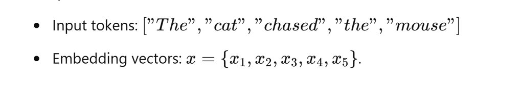
but first of all, why the MLP is not enough, we need self-attention mechanism??? for example, Let’s analyze the sentence:

“The cat, which was very hungry, chased the mouse.”

and compare how a plain MLP and an MLP with self-attention process this example mathematically. The focus will be on how self-attention computes the relationships between words like “cat,” “hungry,” “chased,” and “mouse.”

To fully understand the mechanism of self-attention, let’s start from the toy example in this clip and colab.

First, “causal running average” as illustrated by below codes, it ensures that information from future time steps does not influence the current position ttt, preserving the temporal structure. This is often used in tasks where each time step ttt can only depend on past or present information, such as in autoregressive models or attention mechanisms.

torch.manual_seed(1337)
B,T,C = 4,8,2 # batch, time, channels
x = torch.randn(B,T,C)
x.shape

# We want x[b,t] = mean_{i<=t} x[b,i]
xbow = torch.zeros((B,T,C))
for b in range(B):
    for t in range(T):
        xprev = x[b,:t+1] # (t,C)
        xbow[b,t] = torch.mean(xprev, 0)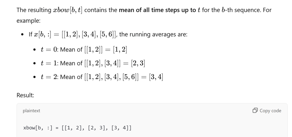

Second, version 2, use matrix multiply for a weighted aggregation, it accomplish the same as above but in matrix computation, neat.

# version 2: using matrix multiply for a weighted aggregation
wei = torch.tril(torch.ones(T, T))
wei = wei / wei.sum(1, keepdim=True)
xbow2 = wei @ x # (B, T, T) @ (B, T, C) ----> (B, T, C)
torch.allclose(xbow, xbow2)

Now, use self-attention

# version 4: self-attention!
torch.manual_seed(1337)
B,T,C = 4,8,32 # batch, time, channels
x = torch.randn(B,T,C)

# let's see a single Head perform self-attention
head_size = 16
key = nn.Linear(C, head_size, bias=False)
query = nn.Linear(C, head_size, bias=False)
value = nn.Linear(C, head_size, bias=False)
k = key(x)   # (B, T, 16)
q = query(x) # (B, T, 16)
wei =  q @ k.transpose(-2, -1) # (B, T, 16) @ (B, 16, T) ---> (B, T, T)

tril = torch.tril(torch.ones(T, T))
#wei = torch.zeros((T,T))
wei = wei.masked_fill(tril == 0, float('-inf'))
wei = F.softmax(wei, dim=-1)

v = value(x)
out = wei @ v
#out = wei @ x

out.shape

Input: A batch of sequences represented by embeddings (B,T,CB, T, CB,T,C). Output: Contextualized representations for each token in the sequence.

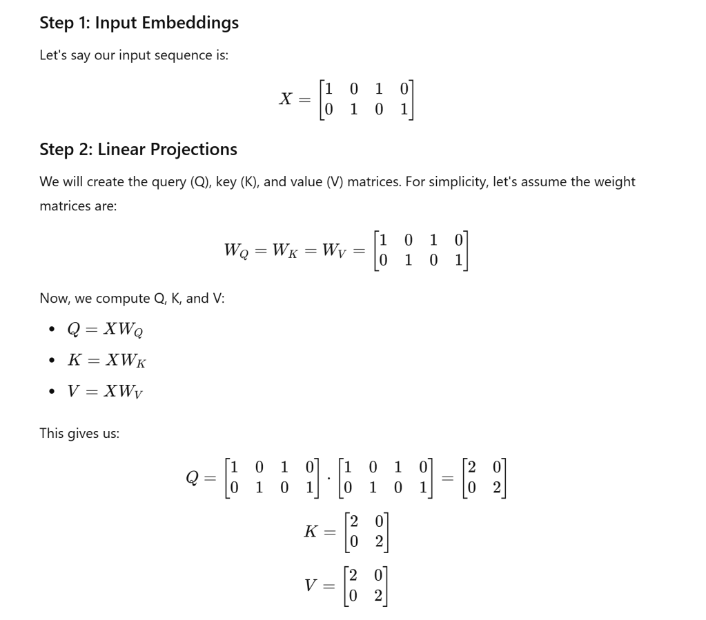
The Queries (Q), Keys (K), and Values (V) are not pre-defined concepts but are learned through training. Let’s break down the step-by-step process of how these components are created and learned during the training of a transformer model.

It’s used to project x into Q, K V respective spaces by multiplying random i.e. unlearned matrix Wq, Wk and Wv. Example:

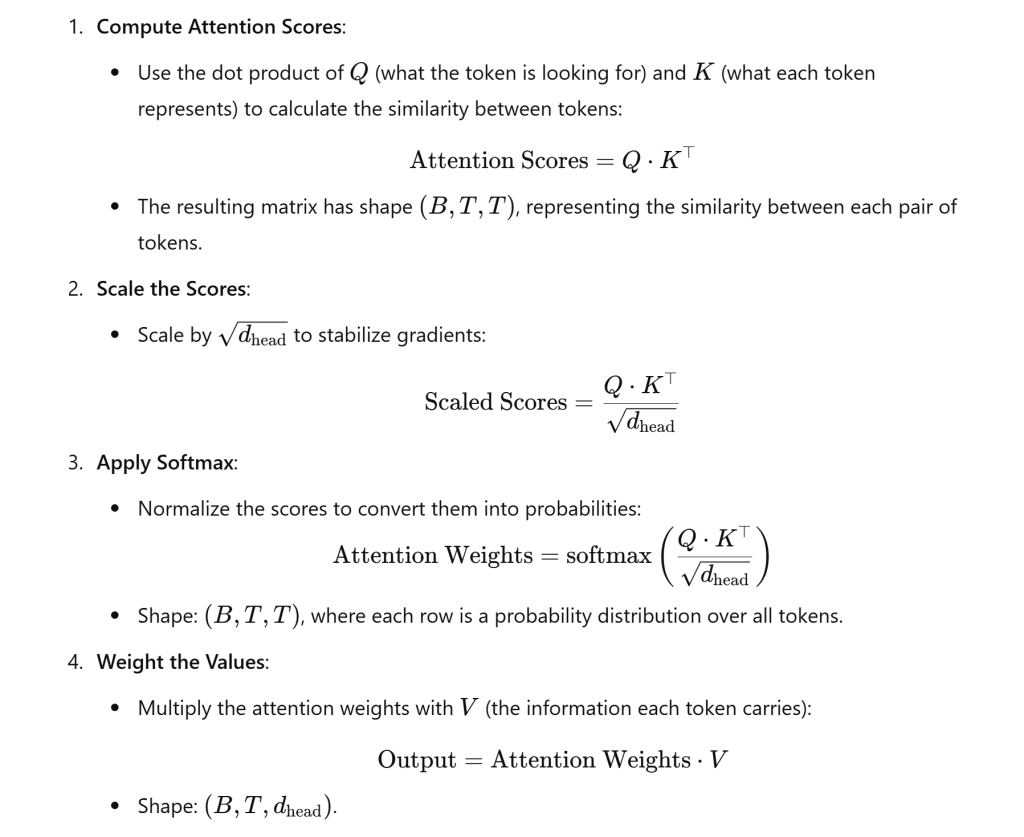
in this example Attention calculates how tokens interact (e.g., “cat” attends to “chased”). Over time, this process refines the Q, K, V representations to capture meaningful relationships within the data.

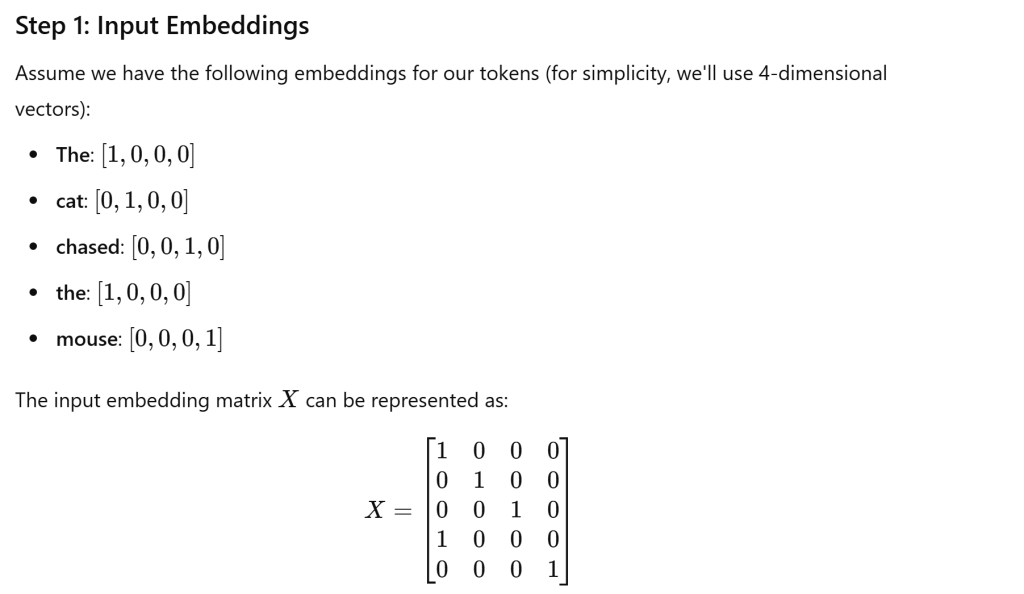
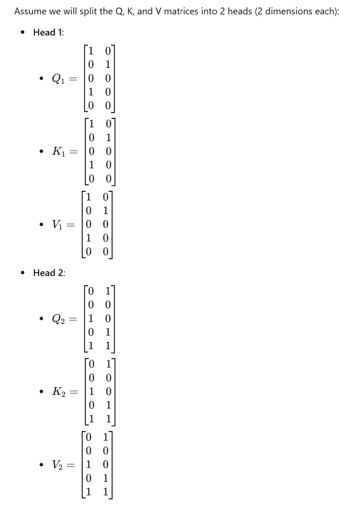
To clarify the split and organization of data, let’s use a very simple example, input embeddings: Let’s assume we have a sequence of 2 tokens, each represented by a 4-dimensional embedding. For simplicity, we will use small values for the embeddings. Number of heads: We will use 2 heads. Output dimension: The output dimension per head will be 2 (since the total output dimension will be 4, divided by 2 heads).

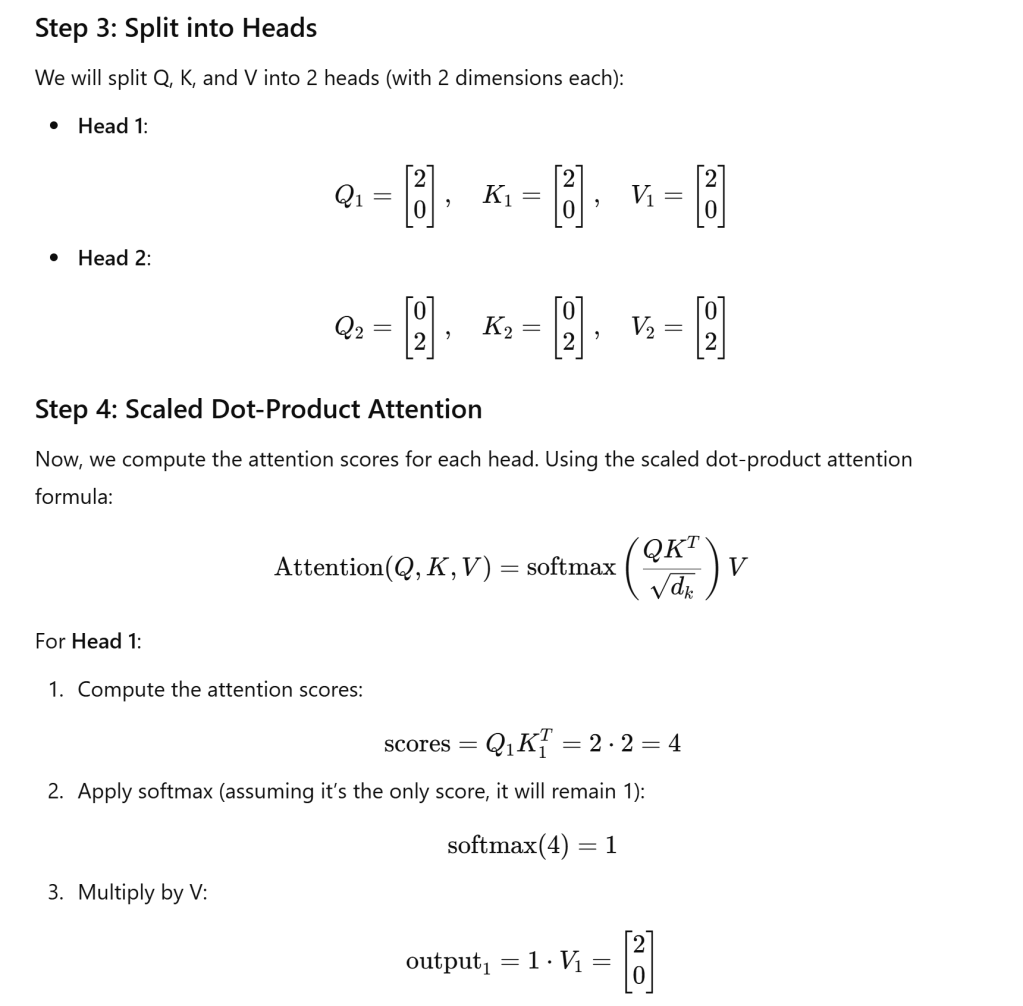
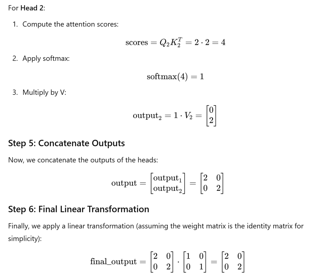
In this simplified example, we demonstrated how input embeddings are transformed into Q, K, and V matrices, how they are split into heads, how attention is computed for each head, and how the outputs are concatenated and transformed back to the final output.

Now let’s use “the cat chased the mouse”, a more complicated example to illustrate.

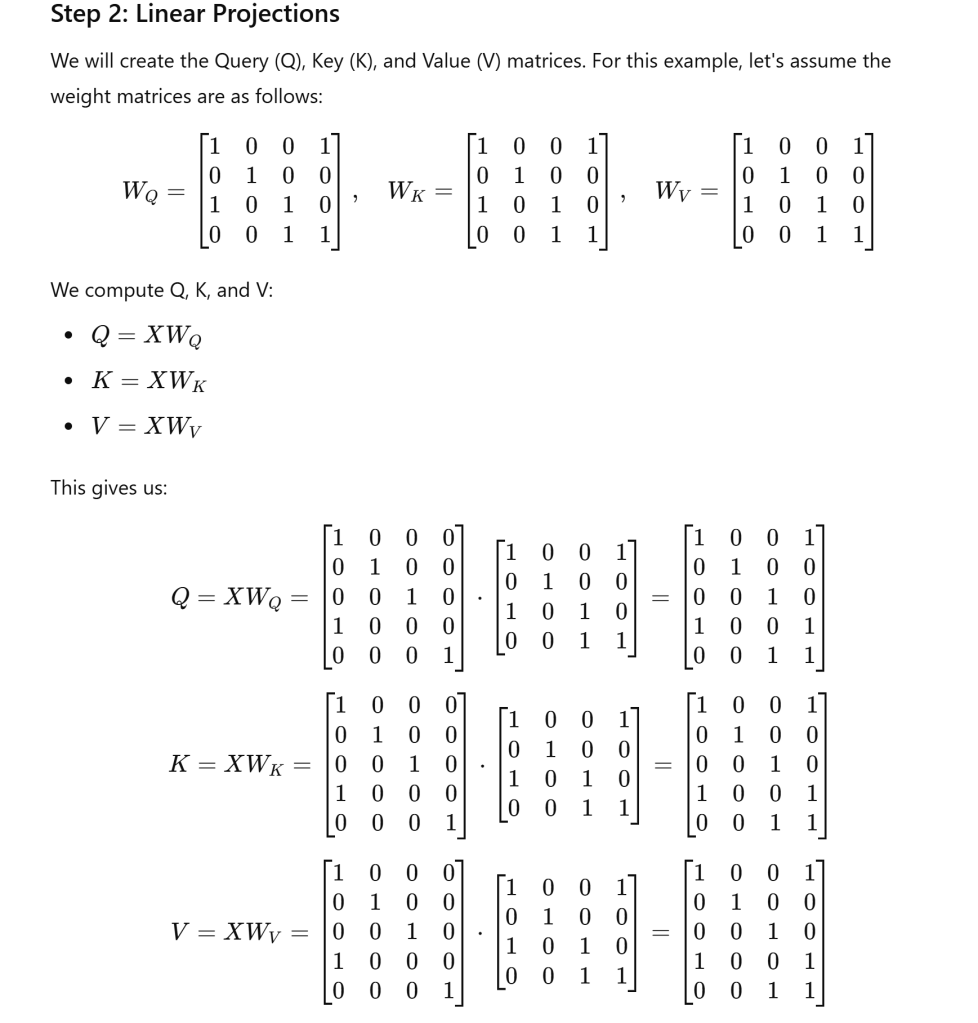
When we compute the Q, K, and V matrices from the input embeddings, we effectively transform these embeddings into representations that can be compared to one another. Query (Q) represents the word looking for relevant information. Key (K) represents the word that contains information. Value (V) carries the information that the model will return based on the attention scores.

Splitting attention into multiple heads allows models to learn diverse and rich representations of the input data, improving their ability to capture complex relationships, reduce computational load, and enhance generalization. This architectural choice has proven to be highly effective in natural language processing and other tasks.

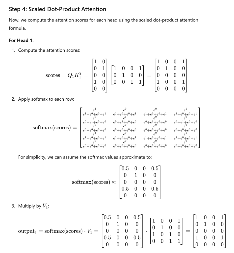
First Row (Output for “The”):

• [1,0,0,1][1, 0, 0, 1][1,0,0,1]: This row indicates some level of attention but isn’t directly relevant to “cat” or “mouse.”

Second Row (Output for “cat”):

• [0,1,0,1][0, 1, 0, 1][0,1,0,1]: This row indicates that the representation for “cat” has significant contributions from the “the” context, reflected in the last two entries. The second entry corresponds to the representation of “cat,” which is a focus point.

Third Row (Output for “chased”):

• [0,0,0,0][0, 0, 0, 0][0,0,0,0]: Indicates that “chased” may not have much relevance in the attention context we are analyzing, or it’s not actively contributing to the immediate representation regarding “cat” and “mouse.”

Fourth Row (Output for “the”):

• [1,1,0,1][1, 1, 0, 1][1,1,0,1]: This row reflects contributions from both “cat” and “mouse,” indicating that “the” is likely capturing context from both entities.

Fifth Row (Output for “mouse”):

• [0,0,0,0][0, 0, 0, 0][0,0,0,0]: Similar to “chased,” this row indicates low attention for “mouse” in this specific context.

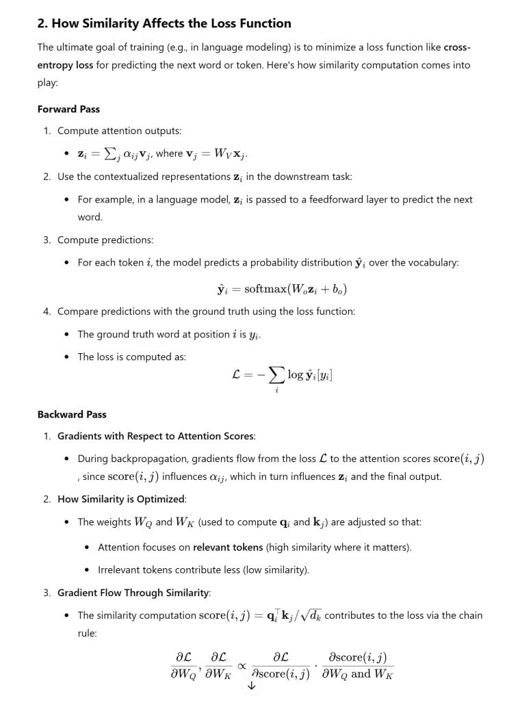
The next question, in this seemingly artifact/designing of K, Q, V self-attention mechanism, how are they optimized, or to be more specific, how are their values iteratively updated with some learning rate in minimizing a loss function?

It’s worth noting that self-attention is not computed across examples within a batch. It is computed independently for each example in the batch. Each sequence in the batch undergoes its own self-attention computation, ensuring that tokens within a sequence interact with each other, but there is no interaction between sequences in the batch. like in below example, B = 4, T = 8, which is also block_size, self-attention is independently computed each block_size or each T.

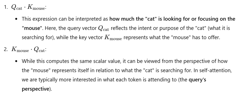
I notice the Q and K is interchangeable from math perspective, but Interpretability: While QQQ and KKK are mathematically interchangeable, their distinct roles provide interpretability:

Keys represent the “information” aspect available for that search. Queries represent the “search” or “inquiry” aspect.

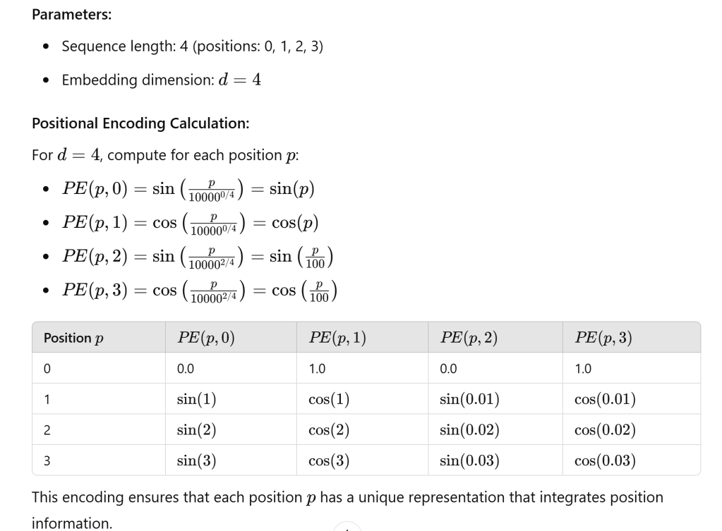
Lastly, knowing contextual relationship is not enough, positioning is also important, how does AI expert figure out positioning using linear algebra to understand the order of words in a sequence.?

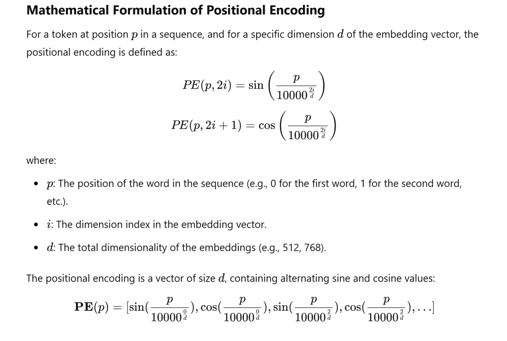
Here is an example to illustrate

While 10000 is somewhat arbitrary, it is a deliberate choice aimed at balancing the scale of positional encodings with the token embeddings. Variations of positional encoding exist (e.g., learned positional embeddings), but the sinusoidal encoding with the 10000 denominator has become a standard in the original Transformer architecture due to its effectiveness.

While the summary above brings me very close to fully understanding K, Q, and V, the video by Serrano.Academy is absolutely outstanding!

Kudos to Google Brain who came up with this ground-breaking paper “attention is all you need”!

below is the full codes in implementing GPT by Andrej:

import torch
import torch.nn as nn
from torch.nn import functional as F

# hyperparameters
batch_size = 16 # how many independent sequences will we process in parallel?
block_size = 32 # what is the maximum context length for predictions?
max_iters = 5000
eval_interval = 100
learning_rate = 1e-3
device = 'cuda' if torch.cuda.is_available() else 'cpu'
eval_iters = 200
n_embd = 64
n_head = 4
n_layer = 4
dropout = 0.0
# ------------

torch.manual_seed(1337)

# wget https://raw.githubusercontent.com/karpathy/char-rnn/master/data/tinyshakespeare/input.txt
with open('input.txt', 'r', encoding='utf-8') as f:
    text = f.read()

# here are all the unique characters that occur in this text
chars = sorted(list(set(text)))
vocab_size = len(chars)
# create a mapping from characters to integers
stoi = { ch:i for i,ch in enumerate(chars) }
itos = { i:ch for i,ch in enumerate(chars) }
encode = lambda s: [stoi[c] for c in s] # encoder: take a string, output a list of integers
decode = lambda l: ''.join([itos[i] for i in l]) # decoder: take a list of integers, output a string

# Train and test splits
data = torch.tensor(encode(text), dtype=torch.long)
n = int(0.9*len(data)) # first 90% will be train, rest val
train_data = data[:n]
val_data = data[n:]

# data loading
def get_batch(split):
    # generate a small batch of data of inputs x and targets y
    data = train_data if split == 'train' else val_data
    ix = torch.randint(len(data) - block_size, (batch_size,))
    x = torch.stack([data[i:i+block_size] for i in ix])
    y = torch.stack([data[i+1:i+block_size+1] for i in ix])
    x, y = x.to(device), y.to(device)
    return x, y

@torch.no_grad()
def estimate_loss():
    out = {}
    model.eval()
    for split in ['train', 'val']:
        losses = torch.zeros(eval_iters)
        for k in range(eval_iters):
            X, Y = get_batch(split)
            logits, loss = model(X, Y)
            losses[k] = loss.item()
        out[split] = losses.mean()
    model.train()
    return out

class Head(nn.Module):
    """ one head of self-attention """

    def __init__(self, head_size):
        super().__init__()
        self.key = nn.Linear(n_embd, head_size, bias=False)
        self.query = nn.Linear(n_embd, head_size, bias=False)
        self.value = nn.Linear(n_embd, head_size, bias=False)
        self.register_buffer('tril', torch.tril(torch.ones(block_size, block_size)))

        self.dropout = nn.Dropout(dropout)

    def forward(self, x):
        B,T,C = x.shape
        k = self.key(x)   # (B,T,C)
        q = self.query(x) # (B,T,C)
        # compute attention scores ("affinities")
        wei = q @ k.transpose(-2,-1) * C**-0.5 # (B, T, C) @ (B, C, T) -> (B, T, T)
        wei = wei.masked_fill(self.tril[:T, :T] == 0, float('-inf')) # (B, T, T)
        wei = F.softmax(wei, dim=-1) # (B, T, T)
        wei = self.dropout(wei)
        # perform the weighted aggregation of the values
        v = self.value(x) # (B,T,C)
        out = wei @ v # (B, T, T) @ (B, T, C) -> (B, T, C)
        return out

class MultiHeadAttention(nn.Module):
    """ multiple heads of self-attention in parallel """

    def __init__(self, num_heads, head_size):
        super().__init__()
        self.heads = nn.ModuleList([Head(head_size) for _ in range(num_heads)])
        self.proj = nn.Linear(n_embd, n_embd)
        self.dropout = nn.Dropout(dropout)

    def forward(self, x):
        out = torch.cat([h(x) for h in self.heads], dim=-1)
        out = self.dropout(self.proj(out))
        return out

class FeedFoward(nn.Module):
    """ a simple linear layer followed by a non-linearity """

    def __init__(self, n_embd):
        super().__init__()
        self.net = nn.Sequential(
            nn.Linear(n_embd, 4 * n_embd),
            nn.ReLU(),
            nn.Linear(4 * n_embd, n_embd),
            nn.Dropout(dropout),
        )

    def forward(self, x):
        return self.net(x)

class Block(nn.Module):
    """ Transformer block: communication followed by computation """

    def __init__(self, n_embd, n_head):
        # n_embd: embedding dimension, n_head: the number of heads we'd like
        super().__init__()
        head_size = n_embd // n_head
        self.sa = MultiHeadAttention(n_head, head_size)
        self.ffwd = FeedFoward(n_embd)
        self.ln1 = nn.LayerNorm(n_embd)
        self.ln2 = nn.LayerNorm(n_embd)

    def forward(self, x):
        x = x + self.sa(self.ln1(x))
        x = x + self.ffwd(self.ln2(x))
        return x

# super simple bigram model
class BigramLanguageModel(nn.Module):

    def __init__(self):
        super().__init__()
        # each token directly reads off the logits for the next token from a lookup table
        self.token_embedding_table = nn.Embedding(vocab_size, n_embd)
        self.position_embedding_table = nn.Embedding(block_size, n_embd)
        self.blocks = nn.Sequential(*[Block(n_embd, n_head=n_head) for _ in range(n_layer)])
        self.ln_f = nn.LayerNorm(n_embd) # final layer norm
        self.lm_head = nn.Linear(n_embd, vocab_size)

    def forward(self, idx, targets=None):
        B, T = idx.shape

        # idx and targets are both (B,T) tensor of integers
        tok_emb = self.token_embedding_table(idx) # (B,T,C)
        pos_emb = self.position_embedding_table(torch.arange(T, device=device)) # (T,C)
        x = tok_emb + pos_emb # (B,T,C)
        x = self.blocks(x) # (B,T,C)
        x = self.ln_f(x) # (B,T,C)
        logits = self.lm_head(x) # (B,T,vocab_size)

        if targets is None:
            loss = None
        else:
            B, T, C = logits.shape
            logits = logits.view(B*T, C)
            targets = targets.view(B*T)
            loss = F.cross_entropy(logits, targets)

        return logits, loss

    def generate(self, idx, max_new_tokens):
        # idx is (B, T) array of indices in the current context
        for _ in range(max_new_tokens):
            # crop idx to the last block_size tokens
            idx_cond = idx[:, -block_size:]
            # get the predictions
            logits, loss = self(idx_cond)
            # focus only on the last time step
            logits = logits[:, -1, :] # becomes (B, C)
            # apply softmax to get probabilities
            probs = F.softmax(logits, dim=-1) # (B, C)
            # sample from the distribution
            idx_next = torch.multinomial(probs, num_samples=1) # (B, 1)
            # append sampled index to the running sequence
            idx = torch.cat((idx, idx_next), dim=1) # (B, T+1)
        return idx

model = BigramLanguageModel()
m = model.to(device)
# print the number of parameters in the model
print(sum(p.numel() for p in m.parameters())/1e6, 'M parameters')

# create a PyTorch optimizer
optimizer = torch.optim.AdamW(model.parameters(), lr=learning_rate)

for iter in range(max_iters):

    # every once in a while evaluate the loss on train and val sets
    if iter % eval_interval == 0 or iter == max_iters - 1:
        losses = estimate_loss()
        print(f"step {iter}: train loss {losses['train']:.4f}, val loss {losses['val']:.4f}")

    # sample a batch of data
    xb, yb = get_batch('train')

    # evaluate the loss
    logits, loss = model(xb, yb)
    optimizer.zero_grad(set_to_none=True)
    loss.backward()
    optimizer.step()

# generate from the model
context = torch.zeros((1, 1), dtype=torch.long, device=device)
print(decode(m.generate(context, max_new_tokens=2000)[0].tolist()))